Wolfram Cloud Document

A tree-ring cross-section whose ring widths ARE the regional master chronology grows one year at a time, while the reconstructed (tan) and observed (red) summer temperatures are drawn beside it. The two track each other for a century – then, after 1960, the thermometers pull away from what the rings record. That gap is the divergence problem.

A tree growing at the edge of where trees can grow keeps a diary. Each summer it lays down a ring; in a place cold enough that warmth is the thing in shortest supply, a warm summer buys a wide, dense ring and a cool one a thin, soft ring. Stack up enough trees, cross-date them so every ring sits in its true calendar year, and you can read a centuries-long record of summer temperature off the wood – long before any thermometer existed. This is dendroclimatology, and it underpins a large fraction of what we know about climate over the last one to two thousand years.

This post does the whole thing from scratch in the Wolfram Language, for one of the best-studied temperature-sensitive regions on Earth: the Scots-pine treeline of northern Fennoscandia (Lapland, around 68°N). We download raw ring measurements from the International Tree-Ring Data Bank, remove the growth trend every tree carries simply from getting older, average the trees into a master chronology, check that they are really telling a common story, find which season they record, and calibrate them against the instrumental temperature record. Then we confront the awkward part that most popular accounts skip: since about 1960 these trees have recorded LESS warming than the thermometers measured. That is the famous divergence problem, and meeting it honestly is the point of the post.

Everything lives in a companion package, DendroX.wl – the only file you need beside this notebook. Every step below is a one-liner whose call sits directly above its (pre-computed) output; evaluate the notebook and it fetches its own data and rebuilds every figure. No data files to download by hand, no API key.

1. Setup: one call builds the whole network

Load the package and build the network. dxBuildNetwork[] downloads the ring-width and density measurements for ten Pinus sylvestris sites (plus Grudd's millennium-long Torneträsk chronology) and the HadCRUT5 instrumental temperature, then parses, detrends, builds both master chronologies, calibrates and reconstructs – returning a single association. (Shown pre-computed; evaluate to rebuild live, ~1–2 minutes.)

SetDirectory[NotebookDirectory[]];Get["DendroX.wl"];net=dxBuildNetwork[];(*fetchITRDB+HadCRUT5,buildeverything*)

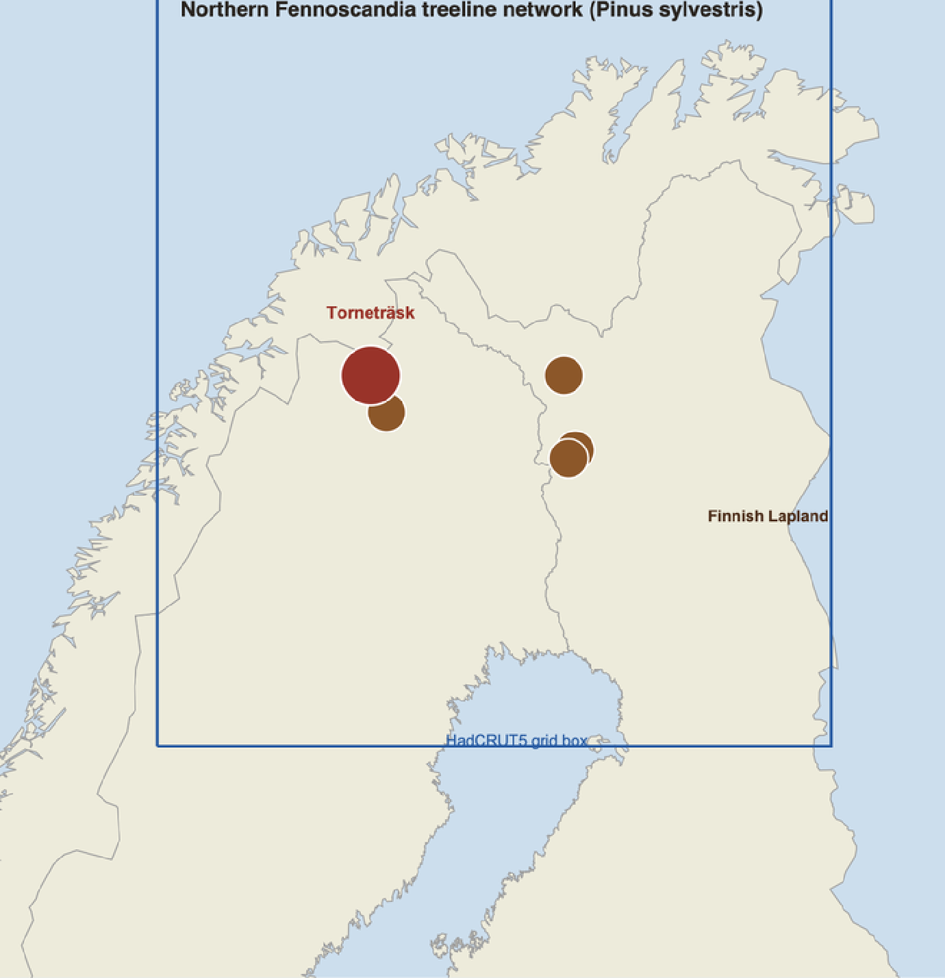
The ten core sites cluster along the Swedish–Finnish treeline north of the Arctic Circle, where the dashed box marks the temperature grid we will calibrate against. This is not a random pile of chronologies: temperature-sensitive sites are chosen deliberately, because the whole method rests on the trees being limited by the one thing we want to reconstruct.

dxFigMap[net]

2. From a tree to a number

A raw ITRDB measurement file (the decades-old "Tucson" format) is a list of ring widths, in hundredths or thousandths of a millimetre, one core per series, packed into fixed columns. The package reads them into tidy per-core associations. But you cannot simply average raw widths, because of one dominant, entirely non-climatic effect: a young tree builds wide rings over its small core and lays down progressively narrower ones as the same volume of wood spreads over an ever-larger circumference. Plot every core against its own age and the trend leaps out – a steep early decline common to all of them.

dxFigAgeTrend[net]

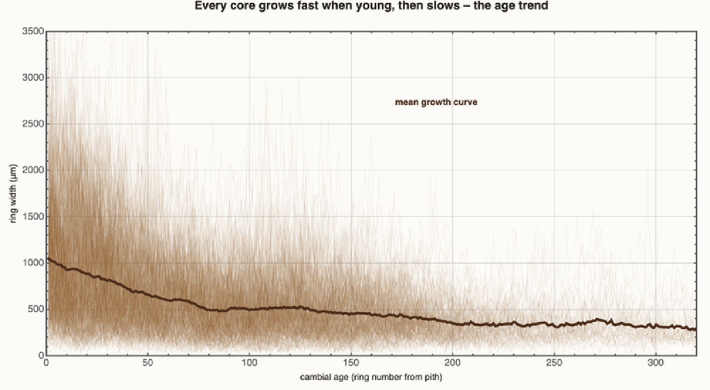
That shared curve is biology, not climate. If we averaged raw widths, sites with many young trees would look "warm" purely because young trees grow fast. Removing this age trend – standardization – is the central craft of dendrochronology, and the next step.

3. Standardization: dividing out the growth curve

For each core we fit a smooth growth curve and divide the raw widths by it. The conservative classic is the modified negative exponential: a negative-exponential decay where a young tree's early surge calls for one, and a straight line otherwise (as for the slowly-declining core shown here). The result is a dimensionless ring-width index that fluctuates around 1: above 1 means "wider than this tree's age would predict", below 1 means "narrower". The age trend is gone; what remains is the year-to-year climate signal, on a common scale for every tree regardless of age or size.

dxFigDetrend[net]

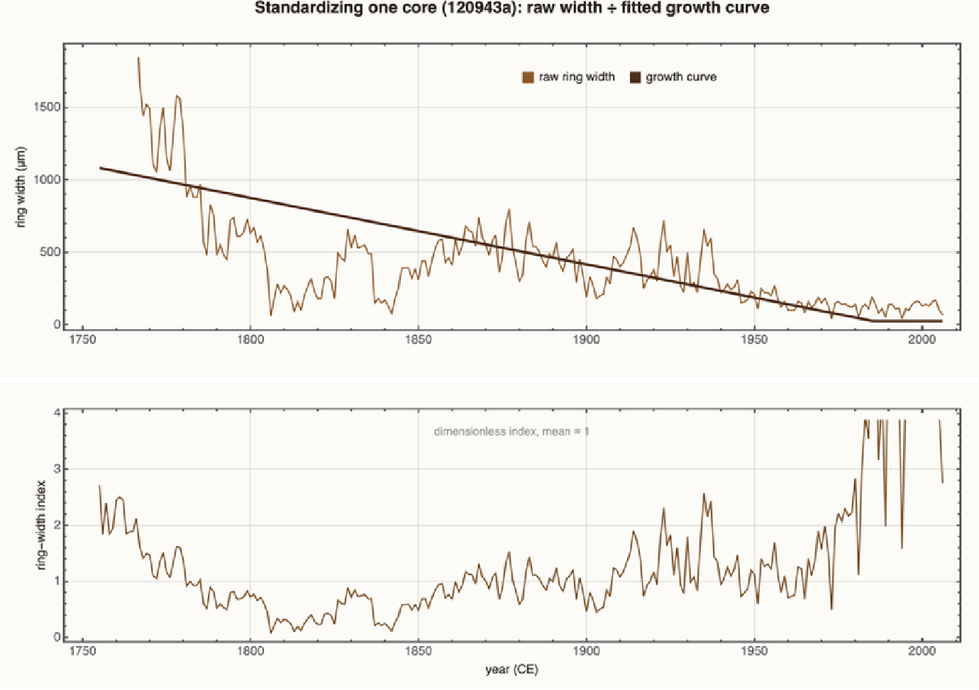
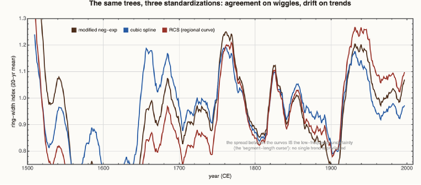
Standardization is a double-edged knife. A stiff curve (negative exponential, or the regional-curve method dxRCS that this package also implements) preserves slow, century-scale swings – which is what we want for climate – but a flexible spline would scrub them out along with the age trend. Because each core is only so long, there is a hard limit on the lowest frequency any single tree can preserve (the "segment-length curse"). We keep the detrending deliberately conservative, and check below how much low-frequency signal survives.

This is not hand-waving; you can watch it happen. Build the very same chronology three ways – modified negative exponential, a flexible cubic spline, and regional-curve standardization – and overlay them. They agree almost perfectly on the year-to-year and decadal wiggles, but they drift apart on the slow, century-scale trends, precisely the band the spline quietly removes. The spread between the curves is not error in any one of them; it is the genuine low-frequency uncertainty of the method, and it is why this post leans on the conservative choices and shows error bars.

dxFigDetrendEnsemble[net]

4. The master chronology

Now average. For each calendar year we combine the index values of every core that was alive, using a Tukey biweight robust mean so that a single freak ring cannot swing the result. The grey shading is the sample depth – how many cores contribute to each year. It thickens toward the present (more living trees) and thins into the past, which is the fundamental tradeoff of every long chronology: more history, less certainty.

dxFigChronology[net,"TRW"]

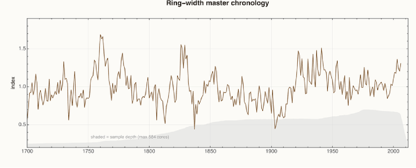
We build the chronology twice, from two different measurements of the same rings: total ring width (above) and maximum latewood density (below) – how dense the hard, dark wood at the outer edge of each ring is. Density is harder to measure but, as we are about to see, a noticeably better thermometer.

dxFigChronology[net,"MXD"]

5. Is the common signal real?

With dozens of cores the density network sits at EPS ≈ 0.99 for the whole period shown – comfortably reliable – even though the underlying inter-series correlation is a more modest ~0.4–0.55. That is the power of replication: pooling many moderately-correlated trees yields a strongly-expressed common signal.

There is a more visceral way to see that common signal – and it is how cross-dating was done by hand for a century: the skeleton plot. Mark each tree's narrowest rings as downward ticks and stack the trees up. Wherever a bad summer struck, every tree wrote a thin ring in the same year, and the ticks line up into vertical 'pointer years' – the anchors that let a dendrochronologist slot an undated piece of wood into absolute calendar time.

Several of the strongest pointer years are not random bad weather. 1837 is the summer after the 1835 Cosigüina eruption, and 1961–1963 brackets Agung – the same volcanic cold snaps we will meet again later, recorded here as synchronized thin rings across the entire forest. The trees agree with each other, and they agree for a reason.

6. What climate do the rings record?

Which month's weather is written into the wood? Correlate the chronology against each calendar month's regional temperature, over the early instrumental period. The answer is unambiguous and physically sensible: a sharp peak in high summer.

Growth at the treeline is limited by the warmth of the few brief weeks when these trees can actually build wood – roughly June through August, peaking in July. Density responds even more cleanly to summer warmth than ring width does. So the natural target to reconstruct is the mean June–August (JJA) temperature, which is what we use from here on.

Which month is only half the question; the other half is where. Correlate the chronology against every cell of the gridded HadCRUT5 temperature field – not just our one box – and the answer is a bullseye: the strongest correlation (r up to ~0.8) sits squarely over the treeline, and fades smoothly outward across Europe. The trees are not picking up some smeared hemispheric average; they are reading the summer temperature of their own corner of the Arctic, which is exactly what a local thermometer should do.

7. Calibration and verification

Now turn the chronology into degrees. We regress observed JJA temperature on the density index over a calibration period (1901–1960) and test the fit honestly on the years we withheld, using the two standard dendro skill scores: the Reduction of Error (RE) and the more demanding Coefficient of Efficiency (CE). Any positive value beats climatology; both come out clearly positive.

Density explains about 59% of the year-to-year variance of summer temperature in the calibration period (ring width, a weaker thermometer, manages ~28%), and the withheld-period RE and CE near 0.38 confirm the relationship is real and transferable, not just an in-sample fit. By the standards of the field this is a good, trustworthy summer-temperature proxy.

8. The reconstruction

Apply the calibration to the whole chronology and we have reconstructed summer temperature – for the network, back to the 1850s; and for Torneträsk's ring-width chronology, across more than a thousand years, complete with the relative warmth around 1000 CE and the cold troughs of the Little Ice Age.

A reconstruction without error bars is a hypothesis dressed as a fact. Two things make the deep past less certain than the present: the calibration coefficients are themselves estimated from a finite sample (so we bootstrap them), and far fewer trees were alive a thousand years ago, so the chronology's signal is noisier where it thins. Propagating both gives an honest 95% band – tight in the well-replicated recent centuries, ballooning back in time exactly where the wood runs out.

This is the prize of dendroclimatology: a year-resolved, absolutely-dated temperature record reaching far beyond the instrumental era, the kind of series that anchors the long temperature reconstructions of the last millennium – now drawn with the candour its sample depth demands. But it rests on one assumption – that the calibration we built on recent decades held in the past. The next section is about exactly where that assumption breaks.

One picture for the road. Strip the axes away and paint each summer a single colour – deep blue for cold, deep red for warm – and a thousand years of reconstruction become a barcode of climate. The blue-shot stretch is the Little Ice Age; the thin instrumental band below blazes red at the right, the recent warmth standing out against everything that came before – and, tellingly, redder than the proxy stripes just above it. That mismatch is the subject of the next section.

9. The divergence problem

Lay the reconstruction over the thermometers. For a century they track beautifully, year for year. Then, from around 1960, something goes wrong: as the real summers warm sharply, the trees keep pace with the wiggles but not with the climb. The reconstruction increasingly falls below the observations – the shaded gap.

This is the divergence problem, first flagged for high-northern-latitude trees by Briffa and colleagues in the late 1990s. It is not subtle here: by the 2000s both the density and ring-width reconstructions under-predict observed summer warming by roughly 1 °C – the trees captured only about half of the warming the thermometers recorded.

Look closely and the failure is specifically a low-frequency one. A running 31-year correlation shows that the year-to-year skill does not collapse – especially for density, the trees still know which summers were warm and which were cool. What they increasingly miss is the trend.

The cleanest way to see it is to plot the gap itself – observed minus reconstructed, smoothed. Flat and near zero through the calibration era, it lifts off through the second half of the 20th century to a persistent positive offset: the trees, year after year, recording less warmth than fell on them.

"After 1960" is a claim, so let us test it instead of asserting it. Two measurements pull apart. A rolling 31-year regression of temperature on the chronology (top) shows the year-to-year sensitivity holding up almost to the present – the trees still know a warm summer from a cool one. But a piecewise-linear model fitted to the gap (bottom) finds a real break around mid-century, after which the gap climbs at about a degree per century, a trend significant at t > 2. So the failure is specific and quantifiable: not a loss of interannual skill, but a slow low-frequency drift in which the trees record steadily less of the warming – exactly the kind of error that is invisible year-to-year yet corrosive to a long reconstruction.

Why would trees stop tracking temperature?

There is no single agreed cause, and that is part of why it matters. The leading hypotheses fall into two families. First, real biology: at some sites warming brings drought stress (warmer air dries the soil, so temperature stops being purely beneficial); 'global dimming' (a mid-century decline in surface sunlight from aerosols) may have throttled photosynthesis; delayed snowmelt, changing seasonality, and nonlinear thresholds have all been proposed. Second, method and data: conservative standardization distorts trends near the ends of chronologies (the very years we care about), the choice of instrumental target carries its own uncertainty at sparse high-latitude stations, and some of the apparent divergence is sensitive to exactly how the chronology is built.

The honest reading of THIS network is nuanced: density holds up better than ring width, the interannual signal largely survives, and the problem is concentrated in the long-term trend. But the consequence is serious and general. If a proxy can under-record a warming it is directly measured against, then it can also have under-recorded past warm periods we cannot check – which complicates any claim that 'the present is unprecedented' built on tree rings alone. Divergence is the reason post-1960 tree-ring data are sometimes truncated or treated separately in large-scale reconstructions, and the reason that honest dendroclimatology now comes with this asterisk attached.

10. Volcanoes written in the rings

A treeline tree is a thermometer, and a thermometer records shocks. The biggest natural shock to summer temperature is an explosive volcanic eruption: it lofts sulfate into the stratosphere, which veils the sun and cools the surface for a few years. If the reconstruction is any good, the great eruptions of the last thousand years should be written into it as cold summers – dated, note, entirely independently, from ice-core sulfate.

They are. Mark the major eruptions – Samalas (1257), Kuwae (1453), Huaynaputina (1601), Laki (1783), Tambora (1815), Krakatoa (1883), Pinatubo (1991) – and the reconstruction dips at them. The superposed-epoch analysis makes it quantitative: averaging the summers around all twenty eruptions, temperature drops below the pre-eruption baseline and stays low for several years, well outside the envelope that random years produce. And the single coldest summer in the whole millennium is 1601 – the year after Huaynaputina, remembered in Russia as the great famine and across the Northern Hemisphere as a year without a summer. The rings did not just track the slow warming; they caught the planet's sharpest cold snaps, and agree with an utterly different archive (polar ice) on when they happened.

11. The hall of fame: extreme summers

With a thousand dated years in hand we can name the record-holders. The fifteen coldest reconstructed summers and the fifteen warmest tell a coherent story: the cold extremes cluster in the depths of the Little Ice Age and in the years after great eruptions (1601, the famine summer after Huaynaputina; 1837 after Cosigüina), while the warm extremes sit overwhelmingly in the medieval centuries around 1000–1100.

And here the post's two themes collide. Read naively, this proxy says the Medieval Warm Period was hotter than today – every one of its warmest summers is medieval, not one is modern. But we have just spent a section showing that these very trees under-record the post-1960 warming. The honest conclusion is not 'the past was warmer' but 'tree rings alone, carrying their divergence, cannot settle the medieval-versus-modern question'. That is precisely why such comparisons are made with many proxies and the instruments together, never with wood alone.

12. The rhythm of the record

A 1900-year record is long enough to ask not just how warm each summer was, but whether the warmth arrives in rhythms. Decompose the reconstruction into its periodic components and a few bands stand out above the red-noise background – a broad multidecadal-to-Gleissberg band around 60–90 years, and a sharp peak near 210 years.

Those are not arbitrary numbers. The ~210-year de Vries (Suess) cycle and the ~88-year Gleissberg cycle are well-known periodicities of solar activity, recorded independently in cosmogenic isotopes; their faint appearance here hints that the Sun leaves a fingerprint on northern summers, while the 60–90 year band also overlaps the multidecadal swings of the North Atlantic. The lower panel – a sliding-window spectrogram – shows these rhythms are not fixed: they strengthen and fade over the centuries, which is exactly why one long, absolutely-dated record is worth so much for finding them.

13. Postscript: from a photograph of a log to a chronology

Everything so far began with numbers someone else had already measured off the wood. But where do those numbers come from? A core or a cross-section, a ruler or a measuring stage, and a great deal of patience. A new generation of public image datasets now lets us do that part too – go straight from a photograph of a tree's cross-section to a dated ring series – so this postscript closes the loop on the other half of the craft. The data here are different (felled plantation Pinus taeda from Uruguay, the UruDendro set), chosen because they come with expert ring delineations to check our work against.

First, find the rings in the image. Segment the wood from the dark bark and background, locate the pith, and unwrap the disc into polar coordinates – angle around, radius outward – where every ring becomes a dark horizontal band and a radial crack becomes a vertical streak that smoothing along the angle simply erases. A global shortest-path trace then follows each dark band all the way around the disc, kept inside the wood; where the bark bites into the disc the outer rings just end there, instead of smearing into it:

Cross-section F02c from the UruDendro dataset (Marichal, Pivato, Randall et al., 2024, Zenodo record 15110647), used and adapted under CC BY 4.0; the cyan ring contours were added by the author.

Each cyan contour sits on a latewood ring, the whole way around – eccentric rings, cracks and bark included. It finds about as many rings as the experts' 22; a single image cannot reliably tell a true annual ring from a strong intra-annual ("false") band, and resolving that is exactly the job of cross-dating, which is next. Precise automatic detection remains an active computer-vision benchmark in its own right (UruDendro; the INBD method of Gillert et al., CVPR 2023), so for the quantitative work below we use the dataset's expert delineations, as a dendrochronologist would at the bench.

There is a second, much simpler way to read the rings – and it is closer to how it is actually done at the bench. Forget tracing whole rings: just walk a single line straight out from the pith and read the darkness of each pixel. Every latewood band is a dark spike, so the rings become peaks in a one-dimensional profile you can literally count. A single line is noisy (the wood has sub-annual wobbles), so we average the darkness around the disc at each radius; the spacings between the peaks ARE the ring widths.

The two methods agree to within a ring or two, which is the reassuring part: a fiddly global contour trace and a one-line darkness profile, built on completely different ideas, count the same rings. The profile is also the more practical of the two for measurement – its peak-to-peak distances give a ring-width series straight away, exactly the input a chronology needs.

How good is "good", quantitatively? Because UruDendro ships expert hand-delineations, we can benchmark both detectors against ground truth. Plot each detected ring radius against the nearest expert ring and the points fall on the 1:1 line: both methods recover about 18 of the 22 annual rings to a median of ~1.5 mm, and the small bias (the detectors mark the dark latewood centre, the experts its outer edge) and the occasional extra ring are exactly the limits we already described.

Cross-dating: the idea that makes it all work

A single tree's ring widths are just a ladder of numbers with no calendar attached. The breakthrough of dendrochronology, Andrew Douglass's insight a century ago, is that trees of the same species in the same climate write the same story: wide in good years, narrow in bad ones, in lockstep. Measure several and their patterns line up. Here are six different trees, each measured from its own photograph, detrended to remove the juvenile growth surge, and dated from the one year we know for certain – 2019, when they were felled:

Once the shared age trend is removed, a real common signal remains (mean inter-tree r ≈ 0.45) – the same wet and dry summers written into every trunk. It is weaker than the treeline pines of the main study would show, and that is the point: these are well-watered plantation trees, only lightly stressed by climate, so their common signal is muted. Strong cross-dating needs trees living at the edge of their tolerance – which is exactly why dendroclimatology goes to the Arctic treeline.

And this is how you date wood that has no felling year – a beam in a medieval roof, the back of a violin, a log in a riverbed. Take one sample's series, slide it year by year against a dated master, and watch for the alignment where the correlation spikes:

The match is unambiguous – a single sharp peak with a Student t near 7, far above the t ≈ 3.5 that dendrochronologists treat as decisive – and it pins the sample's calendar position. (That the peak sits one year off the naive bark-alignment is itself the method earning its keep: it has caught a one-ring discrepancy between samples, a locally-absent or false ring, which is precisely the error cross-dating exists to find.)

One honest gap remains, and it is the obvious next experiment. No public dataset yet pairs a cross-section photograph with that same tree's ITRDB numeric chronology AND a nearby instrumental temperature record. The image half (this section) and the numeric-climate half (sections 1–9) are the two pieces of one machine; bolting them together at a single temperature-limited treeline site – photograph the cores, measure them in the Wolfram Language, cross-date to the regional master, calibrate against the local thermometer – is a project waiting to be done, and nothing in principle stands in the way.

14. What we can and can't claim

What stands up: these treeline pines are genuine summer thermometers. The common signal is strong (EPS ≈ 0.99), the response is cleanly seasonal (a July peak), the calibration is good and verifies out of sample (density r² ≈ 0.59, RE/CE ≈ 0.38), and the resulting reconstruction reproduces the broad strokes of the last millennium. Density is consistently the better proxy than ring width.

What we should not oversell: a single region is not the globe, and one network is not all of dendroclimatology. The reconstruction's low-frequency content is limited by detrending and by segment length, so we quote it as anomalies, not absolute degrees with confidence. Most of all, the post-1960 divergence means the calibration is demonstrably non-stationary – the central uniformitarian assumption of the method fails in the one window where we can test it – so reconstructed values, especially past warm extremes, should be read with that caveat in front of them.

Two analysis choices are worth flagging. Standardization here is conservative (modified negative exponential); the package also provides regional-curve standardization (dxRCS), which preserves more low-frequency signal and is the right tool for the long Torneträsk record. And the chronology is a robust biweight mean of detrended indices, not of raw widths – the distinction matters, and it is what keeps a few anomalous cores from dominating.

15. Reproduce it, and run it on your own forest

There is nothing to reproduce separately – this notebook is the computation. dxBuildNetwork[] downloads its own ITRDB and HadCRUT5 data and rebuilds every figure. The whole pipeline is a handful of public one-liners:

net = dxBuildNetwork[]; (* fetch + build, ~1-2 min *)
dxFigResponse[net] (* which season? *)
dxFigReconstruction[net, "MXD"] (* the divergence *)

To point it at a different region, the building blocks are public: parse any ITRDB file, detrend, pool into a chronology, and calibrate against any temperature series.

series = Flatten[dxParseRWL /@ FileNames["*.rwl", "my_site_folder"]];
det = dxDetrend /@ series; (* or dxRCS[series] *)
chron = dxChronology[det];
dxRunningRbar[det, 30, 10] (* EPS / R-bar through time *)

Pick temperature-limited, high-latitude or high-elevation conifers and you will likely find the same story we found here – a clean summer-temperature signal, and, if your sites run to the present, very possibly its post-1960 fade.

CITE THIS NOTEBOOK

Reading tree rings: Fennoscandia dendroclimatology, summer temperature & the divergence problem
by Marco Thiel
Wolfram Community, STAFF PICKS, June 15, 2026
https://community.wolfram.com/groups/-/m/t/3733750