Abstract: We search for the densest packing of a finite number of hard spheres. The notion of density may be defined in different ways. We may try to minimize the volume of the convex hull or encompassing sphere, or we could try to minimize the potential energy of an attractive force among the spheres. To achieve a solution, we will employ several strategies. Using basic minimization routines, we compute close packings for a few cases of relatively small numbers of spheres, and obtain densities close to, but smaller than, the those for known densest close packings. For the second half of this project, we draw a comparison with existing nuclear-structure data. In particular, we compare binding energies obtained by taking various, tuned, candidate potentials for the inter-nucleon interactions with the true nuclear binding energies.
The problem of close packing of spheres in 3 dimensions has applications in many fields, but it is also one that remains unsolved in the case where the spheres are to be packed into larger, spherical, containers. While existing tabulations of densest known packings serve as numerical lower bounds, true densest packings remain to be found for all but the smallest number of spheres. We explored the feasibility of obtaining a close spherical packing using a simple density-minimization procedure, and found that, for the cases (number of spheres) we tried, our attempts at close-packings produced densities close to, but slightly lower than, those from the tabulated data.
Thereafter, we analyzed the effect of imposing various candidate potentials onto the tabulated sphere packing configurations. The potentials we tried include the Yukawa potential, the Reid nuclear potential (soft-core and hard-core), Coulomb potential and a well potential obtained by adding a centrifugal barrier like term to Coulomb potential. In each case, the parameters appearing in the potential were tuned to minimize the error with respect to the true, mean, binding energies of nuclei with mass numbers from 1 to 72.
Thereafter, we analyzed the effect of imposing various candidate potentials onto the tabulated sphere packing configurations. The potentials we tried include the Yukawa potential, the Reid nuclear potential (soft-core and hard-core), Coulomb potential and a well potential obtained by adding a centrifugal barrier like term to Coulomb potential. In each case, the parameters appearing in the potential were tuned to minimize the error with respect to the true, mean, binding energies of nuclei with mass numbers from 1 to 72.
Assuming the soft-core Reid potential for the inter-nucleon interaction, we generate “binding energies”, corresponding to a given, tentative, close packing of spheres. First we import data on spherical close packing:
In[]:=
packingData=Import["http://www.randomwalk.de/sphere/insphr/sequences.txt"];
Extract out the features and construct graphics:
In[]:=
StringRecordToPacking[s_String]:=With[{record=Map[ToExpression,Map[StringSplit,StringSplit[s,"\n"]],-1]},<|"Count"First[record][[1]],"Radius"1First[record][[2]],"Density"First[record][[1]],"Centers"Rest[record]〚All,2;;4〛,"Graphics3D"Graphics3D[{Ball[Map[Rest,Rest[record]],First[record][[2]]],{Opacity[0.5],Sphere[{0,0,0},1]}},BoxedFalse]|>]
3
First[record][[2]]
data=Dataset[MapIndexed[(First[#2]StringRecordToPacking[#1])&,Take[StringSplit[StringDrop[packingData,3791],"\n\n"],72]]];RandomChoice[data]//Values
Out[]=
Count4,Radius2.22474,Density0.363261,Centers{{-0.259513,-0.44949,-0.183503},{0.519026,-5.99576×,-0.183503},{-0.259513,0.44949,-0.183503},{-3.23374×,1.03795×,0.55051}},Graphics3D
-8
10
-9
10
-8
10
Extracting the densities from this dataset,
densities=Table[(Values/@data)〚n〛["Density"],{n,Length[data]}]
Out[]=
{1.,0.25,0.299889,0.363261,0.355339,0.426407,0.402317,0.432166,0.441343,0.440055,0.450039,0.490951,0.481481,0.473991,0.48375,0.481172,0.485634,0.492329,0.489425,0.477214,0.495571,0.47955,0.481836,0.479467,0.49862,0.494062,0.486879,0.493865,0.4976,0.499378,0.502715,0.50474,0.508005,0.512681,0.513667,0.517404,0.51589,0.52873,0.517498,0.51911,0.516995,0.525266,0.521361,0.522623,0.525754,0.525145,0.524773,0.528056,0.530899,0.530647,0.532383,0.530841,0.536258,0.536078,0.534811,0.541679,0.537813,0.54083,0.544523,0.551124,0.557758,0.547848,0.550373,0.544035,0.544364,0.544878,0.545841,0.544018,0.546072,0.549057,0.54466,0.544502}
we note the kinks therein -- that is, for certain numbers of spheres, the density of the close pack is locally maximum.
ListLinePlot[densities,PlotMarkers{Automatic,5},PlotRange{All,{0,0.8}},AxesLabel{"Number of spehres","Close pack densities"}]
Out[]=
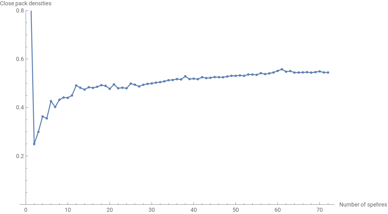
This happens when packing a number of spheres belonging to the following list of the positions of the 22 kinks:
kinks=Table[If[densities〚i〛>densities〚i+1〛&&densities〚i〛>densities〚i-1〛,i,Nothing],{i,2,Length[data]-1}]
Out[]=
{4,6,9,12,15,18,21,23,25,36,38,40,42,45,49,51,53,56,61,63,67,70}
Length[kinks]
Out[]=
22
Comparing this with magic numbers in nuclear structure, we see that close packing of the magic or doubly magic numbers of spheres (4, 36, 40, 56 and 70) corresponds to kinks in the density plot. The rest of the kinks in densities do not belong to the list of nuclear magic (or doubly magic) numbers.
magicNumbers={2,8,20,28,50,82,126}doublyMagicNumbers=Cases[DeleteDuplicates@Sort[Total/@Tuples[magicNumbers,2]],x_/;x<72]
Out[]=
{2,8,20,28,50,82,126}
Out[]=
{4,10,16,22,28,30,36,40,48,52,56,58,70}
Intersection[Union[magicNumbers,doublyMagicNumbers],kinks]
Out[]=
{4,36,40,56,70}
In[]:=
GetCenters[n_]:=Values[data[n]]["Centers"]
In[]:=
$Assumptions={{h,μ,m}∈Reals};
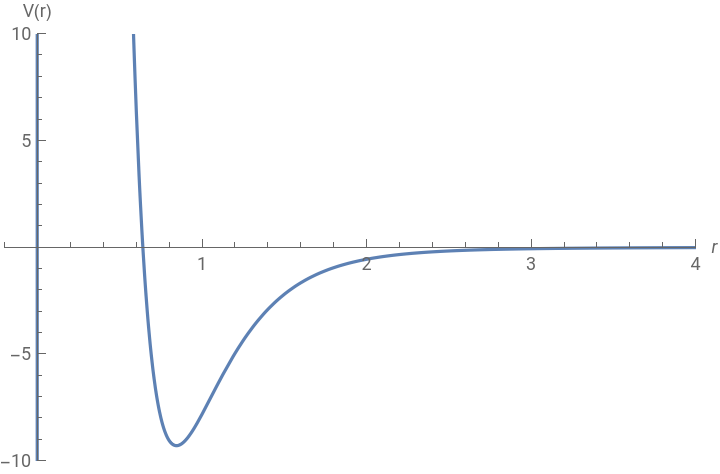
ReidPotential["Soft-Core"][r_Real,μ_:0.7,h_]:=-h+157.76-619.54Plot[ReidPotential["Soft-Core"][r,0.7,1],{r,-0.2,6},PlotRange{{-0.2,4},{-10,10}},AxesLabel{r,"V(r)"}]
-μr
μr
-4μr
μr
-7μr
μr
Out[]=
In[]:=
ConfigBE[centers_List,μ_,h_]:=With{nSpheres=Length[centers]},r[i_Integer,j_Integer]:=EuclideanDistance[centers〚i〛,centers〚j〛];totalPE=ReidPotential["Soft-Core"][r[i,j],μ,h];-totalPEnSpherespackedSpheresSoftCoreReidBE[μ_,h_]:=Table[ConfigBE[GetCenters[n],μ,h],{n,72}]
nSpheres
∑
i=1
nSpheres
∑
j=i+1
Next, we import data on nuclear binding energies:
nuclearStructureDataMeanBE=Quiet@Table[Mean@EntityValue[EntityList[EntityClass["Isotope",{"MassNumber"A}]],"BindingEnergy"],{A,294}];ListPlot[nuclearStructureDataMeanBE,AxesLabel{"Mass Number(A)","Binding Energy (MeV/Nucleon)"}]
Out[]=
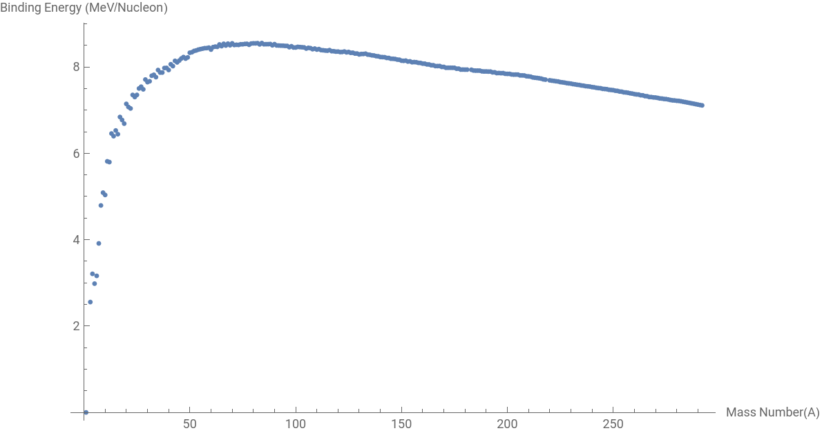
This operation is repeated for multiple candidate potentials, leading to the following variation of the binding energies for the various potentials.
We see that with tuning the parameters in the potential, the densest known packings of spheres come closest to reproducing the nuclear binding energy curve in the case of the soft-core Reid potential.