Introduction
Introduction
An attractor is called strange if it has a fractal structure, that is if it has non-integer Hausdorff dimension. This is often the case when the dynamics on it are chaotic, but strange nonchaotic attractors also exist. If a strange attractor is chaotic, exhibiting sensitive dependence on initial conditions, then any two arbitrarily close alternative initial points on the attractor, after any of various numbers of iterations, will lead to points that are arbitrarily far apart (subject to the confines of the attractor), and after any of various other numbers of iterations will lead to points that are arbitrarily close together. Thus a dynamic system with a chaotic attractor is locally unstable yet globally stable: once some sequences have entered the attractor, nearby points diverge from one another but never depart from the attractor.
The term strange attractor was coined by David Ruelle and Floris Takens to describe the attractor resulting from a series of bifurcations of a system describing fluid flow. Strange attractors are often differentiable in a few directions, but some are like a Cantor dust, and therefore not differentiable. Strange attractors may also be found in the presence of noise, where they may be shown to support invariant random probability measures of Sinai–Ruelle–Bowen type.
Examples of strange attractors include the Rössler attractor, and Lorenz attractor.
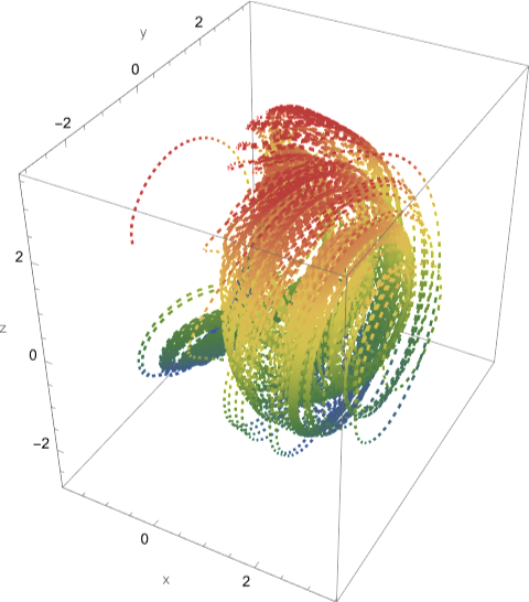
Aizawa Attractor
Aizawa Attractor
Define parameters for the Aizawa Attractor
parameters={a0.95,b0.7,c0.6,d3.5,e0.25,f0.1};
Define the system of differential equations
equations={x'[t]==(z[t]-b)x[t]-dy[t],y'[t]==dx[t]+(z[t]-b)y[t],z'[t]==c+az[t]-z[t]^3/3-(x[t]^2+y[t]^2)(1+ez[t])+fz[t]x[t]^3}/.parameters;
Initial conditions
initialConditions={x[0]==0.1,y[0]==0,z[0]==0};
Time range for the simulation
timeRange={t,0,600};
Solve the system numerically
solution=NDSolve[{equations,initialConditions},{x,y,z},timeRange,Method"LSODA",MaxStepsInfinity];
Plot the attractor’s trajectory in 3D
trajectoryPlotEnhanced=ParametricPlot3D[Evaluate[{x[t],y[t],z[t]}/.solution],{t,0,200},PlotRangeAll,AxesLabel{"x","y","z"},PlotStyle{Dashed},ColorFunction"Rainbow",BoxedTrue,PlotPoints1000];trajectoryPlotEnhanced
Out[]=

Lorenz83
Lorenz83
Parameters for the system
parameters={a0.95,b5.71,f4.83,g4.66};
System of differential equations
equations={x'[t]==-ax[t]-y[t]^2-z[t]^2+af,y'[t]==-y[t]+x[t]y[t]-bx[t]z[t]+g,z'[t]==-z[t]+bx[t]y[t]+x[t]z[t]}/.parameters;
Initial conditions
initialConditions={x[0]==-0.2,y[0]==-2.82,z[0]==2.71};
Numerical solution
solution=NDSolve[{equations,initialConditions},{x,y,z},{t,0,600},Method"StiffnessSwitching"];
3D plot of the attractor with color gradient
trajectoryPlot=ParametricPlot3D[Evaluate[{x[t],y[t],z[t]}/.solution],{t,0,600},PlotRangeAll,AxesLabel{"x","y","z"},PlotStyle{Dashed},ColorFunction"DarkRainbow",ColorFunctionScalingTrue,BoxedTrue,PlotPoints1000];
trajectoryPlot
Plot[{x[t]}/.solution,{t,0,80},PlotStyle{Thickness[0.001],Blue},PlotRangeAll,PlotPoints200,PlotHighlightingNone]
Out[]=
FOUR-WING
FOUR-WING
Parameters for the system
parameters={a0.2,b-0.01,c-0.4};
System of differential equations
equations={x'[t]==ax[t]+y[t]z[t],y'[t]==bx[t]+cy[t]-x[t]z[t],z'[t]==-z[t]-x[t]y[t]}/.parameters;
Initial conditions
initialConditions={x[0]==1.3,y[0]==0.01,z[0]==-0.4};
Numerical solution
solution=NDSolve[{equations,initialConditions},{x,y,z},{t,0,600}];
3D plot of the attractor with color gradient
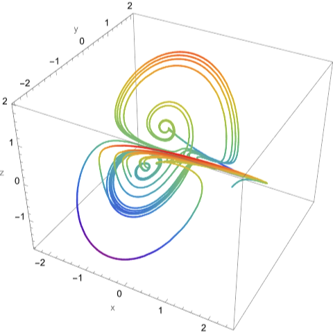
trajectoryPlot=ParametricPlot3D[Evaluate[{x[t],y[t],z[t]}/.solution],{t,0,600},PlotRangeAll,AxesLabel{"x","y","z"},BoxedTrue,PlotStyleThick,ColorFunction"Rainbow",ColorFunctionScalingTrue,PlotPoints1000];
trajectoryPlot
Out[]=
Three-Scroll Unified Chaotic System
Three-Scroll Unified Chaotic System
Adjusted Parameters and Method for Stiff Systems
System of differential equations
Initial conditions
Numerical solution with a different method and reduced time range
3D plot of the attractor
Lorenz2
Lorenz2
Parameters for the system
System of differential equations
Initial conditions
Numerical solution
3D plot of the attractor with color gradient
Double Wing Chaotic Attractor
Double Wing Chaotic Attractor
Parameters for the system
System of differential equations
Initial conditions
Numerical solution
3D plot of the attractor with color gradient
Wang Sun attractor
Wang Sun attractor
Parameters for the system
System of differential equations
Initial conditions
Numerical solution
3D plot of the attractor with color gradient
[TSUCS2] Three-Scroll Unified Chaotic System
[TSUCS2] Three-Scroll Unified Chaotic System
Adjusted Parameters and Method for Stiff Systems
System of differential equations
Initial conditions
Numerical solution with a different method and reduced time range
3D plot of the attractor
References
References
CITE THIS NOTEBOOK
CITE THIS NOTEBOOK
Visualizing chaotic attractors: exploring the intersection of math and art
by Athanasios Paraskevopoulos
Wolfram Community, STAFF PICKS, August 11, 2024
https://community.wolfram.com/groups/-/m/t/3245296
by Athanasios Paraskevopoulos
Wolfram Community, STAFF PICKS, August 11, 2024
https://community.wolfram.com/groups/-/m/t/3245296