ABSTRACT(original article): Wave functions on periodic lattices are commonly described by Bloch band theory. While the focus has traditionally been on periodic structures in flat space, analogous structures in negatively curved hyperbolic space have recently gained attention. However, the resulting “hyperbolic lattices” imply unique challenges on account of the curvature-induced noncommutativity of hyperbolic translations. More precisely, hyperbolic lattices support non-Abelian Bloch states that have so far eluded analytical treatments. In the original research article, we devise a method for the systematic construction of those states by adapting the solid-state-physics notions of supercells and zone folding. We have implemented our method in the freely available Mathematica package HyperBloch. In this Wolfram Mathematica notebook, we demonstrate how HyperBloch can be used to easily apply the supercell method to various tight-binding models, thereby reproducing our results. Additionally, we illustrate how our implementation makes use of the Wolfram language to turn graph and algebraic input data into visualizations of quantities defined on hyperbolic lattices. CITATION (original article): Lenggenhager, P. M., Maciejko, J., and Bzdušek, T. Non-Abelian hyperbolic band theory from supercells. Phys. Rev. Lett. 131, 226401 (2023). DOI: https://doi.org/10.1103/PhysRevLett.131.226401
DATA & CODE: Lenggenhager, P. M., Maciejko, J., and Bzdušek, T. (2023). https://doi.org/10.5281/zenodo.10142168
DATA & CODE: Lenggenhager, P. M., Maciejko, J., and Bzdušek, T. (2023). https://doi.org/10.5281/zenodo.10142168
Introduction
Introduction
While curved spaces are commonly associated with topics such as cosmology and string theory, they are in fact much more common in physics. Of particular interest are spaces with negative curvature. On the one hand, the concept of holography relates such spaces to strongly interacting quantum theories [J. Maldacena, The Large N limit of superconformal field theories and supergravity, Adv. Theor. Math. Phys. 2, 231 (1998)] and on the other hand, hyperbolic lattices, uniform discretizations of the two-dimensional plane with constant negative curvature, have recently gained significant interest. While hyperbolic lattices and various models akin to material models in flat space provide interesting ground for theoretical studies, their experimental realization in metamaterials, including coplanar-waveguide resonators [A. J. Kollár et al., Hyperbolic lattices in circuit quantum electrodynamics. Nature 571, 45 (2019)] and electric-circuit networks [P. M. Lenggenhager et al., Simulating hyperbolic space on a circuit board. Nat. Commun. 13, 4373 (2022)], has elevated them from objects of academic interest to building blocks for engineering metamaterials with potential future applications.
Here, we are interested in exploiting symmetries, in particular the exotic hyperbolic translation symmetry, to study hyperbolic lattices. While there are many similarities between the well-known lattices in flat space and hyperbolic lattices, there are some important conceptual differences. In this context, the similarities are rooted in the presence of a symmetry that can be identified with translations and the validity of a Bloch theorem [J. Maciejko and S. Rayan, Automorphic Bloch theorems for hyperbolic lattices. Proc. Natl. Acad. Sci. U.S.A. 119, e2116869119 (2022)], i.e., a particular set of constraints on the wave functions due to that symmetry. The differences arise from the non-vanishing curvature and its consequence, the noncommutativity of translations. This leads to several challenges in the theoretical description and numerical study of hyperbolic lattices for which various approaches have been developed. In our original research article, we have developed a new approach that resolves many of the issues of previous methods and paves the way for a more complete understanding of hyperbolic lattices.
In this Wolfram notebook, we focus on our implementation of this method in the Mathematica package HyperBloch and how to use it. An accessible introduction to the topic can be found in Part III of the doctoral thesis P.M. Lenggenhager, Emerging avenues in band theory: multigap topology and hyperbolic lattices. https://doi.org/10.3929/ethz-b-000645370 (2023) and the full data and code reproducing the results of the original research article is published in the data and code collection: https://doi.org/10.5281/zenodo.10142168. More details on the software packages can be found in their git repositories: https://github.com/patrick-lenggenhager/HyperCells, https://github.com/patrick-lenggenhager/HyperBloch.
Tight-binding models on hyperbolic lattices
Tight-binding models on hyperbolic lattices
To define translation-invariant tight-binding models on a hyperbolic lattice, we first require the compactified hyperbolic lattice, i.e., the finite lattice with periodic boundary conditions. By definition, a lattice consists of copies of a fundamental unit, the unit cell, generated by discrete translations which form the underlying translation group . Thus, there is a one-to-one correspondence between elements of the translation group and copies of the unit cell. This holds both for infinite lattices (with an infinite translation group) and compactified lattices (with a finite translation group given by the quotient of the full translation group and one of its normal subgroups ). We utilize this relationship to algebraically construct the lattice sites and its nearest-neighbor graph by using the group structure of the relevant translation group to identify nearest neighbors.
Γ
Γ
Γ'
By starting not from the translation group but the full hyperbolic space group , which is a so-called triangle group, one can go even further. The triangle group is a finitely presented group of the form
Δ
|
where are generators corresponding to reflection symmetries at sides of the fundamental triangle with internal angles , , and , , are -, -, -fold rotation symmetries around the corners, respectively. Any triangle group can be conveniently represented by the image of the fundamental Schwarz triangle under all elements of Δ, e.g., for
a,b,c
2π/r
2π/q
2π/p
x=ab
y=bc
z=ca
r
q
p
Δ(2,8,8):
In[]:=
ShowTriangles[{2,8,8},ImageSize250]
Out[]=

A translation group Γ can now be defined to be a normal subgroup of Δ which does neither contain reflections nor elements that taken to some finite power result in the identity. The quotient group takes to role of the point group and its elements (or more precisely the elements of one of its quotients with the appropriate on-site symmetry group) are then in one-to-one correspondence with maximally-symmetric Wyckoff positions within the unit cell. Together, we end up with an algebraic description of all translated copies of the maximally-symmetric Wyckoff positions in the lattice. This allows us to construct more complicated lattices with unit cells that have (symmetric) internal structure.
G=Δ/Γ
We have automated the construction of nearest- and next-nearest-neighbor graphs for arbitrary compactified hyperbolic lattices derived from regular -tessellations in the HyperCells package for GAP, a system for computational discrete algebra. The package also includes a database of quotients based on M. Conder, Quotients of triangle groups acting on surfaces of genus 2 to 101 (2007), https://www.math.auckland.ac.nz/~conder/TriangleGroupQuotients101.txt.
{p,q}
Δ/Γ'
The HyperBloch Mathematica package
The HyperBloch Mathematica package
The output of the HyperCells package can be conveniently imported by its sister package, the HyperBloch package for Mathematica, which is available as a Wolfram paclet.
Installation
Installation
PacletInstall["https://github.com/NCAlgebra/NC/blob/master/NCAlgebra-6.0.3.paclet?raw=true"];PacletInstall["https://github.com/patrick-lenggenhager/HyperBloch/releases/download/v0.9.0/PatrickMLenggenhager__HyperBloch-0.9.0.paclet"];
Please note that NCAlgebra version ≥ 6 is required due to breaking changes in their implementation.
Import the data
Import the data
First, load the package:
In[]:=
Needs["PatrickMLenggenhager`HyperBloch`"]
We consider the case of a single unit cell of the -lattice, i.e., the hyperbolic lattice with eight octagons touching at each site. The output of HyperCells is the text file with the following content:
{8,8}
ShortcellgraphT26String=(*outputfromHyperCellspackage,seehttps://doi.org/10.5281/zenodo.10142168*),5
Out[]//Short=
HyperCells HCC version 1.0[ 2, 8, 8 ][ [ x^2, x*y*z, x*z*y, y^3*z^-1 ], 3 ][ g1, g2, g3, g4 ] -> [ z^-1*x^-1*y*z^-1*y*z*y*x^-1, z^-1*x^-1*y*z^-1*y*z*y*x^-1*y*x*z, z*y*(x^-1*z^-1)^2*y^3*x*z, y^-1…17, 2, 1, g2 ], [ (y^-1*x^-1)^6, (y^-1*x^-1)^6, 20, 3, 0, g3^-1 ], [ (y*x)^5*y, (y*x)^5*y, 20, 3, 1, g3 ], [ (y^-1*x^-1)^7, (y^-1*x^-1)^7, 23, 4, 0, g4^-1 ], [ (y*x)^4*y, (y*x)^4*y, 23, 4, 1, g4 ] ]
which we can easily import using:
In[]:=
cellgraphT26=ImportCellGraphString[cellgraphT26String];
This returns an object with head HCCellGraph containing the relevant information about the cell, its compactification, and the maximally symmetric Wyckoff positions.
This includes the following properties: the triangle group, center of the cell (specified as an integer between 1 and 3 corresponding to Wyckoff positions of type x, y, z), and the genus of the surface on which the cell is compactified:
This includes the following properties: the triangle group, center of the cell (specified as an integer between 1 and 3 corresponding to Wyckoff positions of type x, y, z), and the genus of the surface on which the cell is compactified:
In[]:=
TableForm[{#,ToString@cellgraphT26[#]}&/@{"TriangleGroup","CellCenter","Genus"}]
Out[]//TableForm=
TriangleGroup | {2, 8, 8} |
CellCenter | 3 |
Genus | 2 |
Schwarz triangles
Schwarz triangles
Fundamentally, any cell consists of Schwarz triangles of the corresponding triangle group:
VisualizeCellGraphcellgraphT26,
Out[]=

The Schwarz triangles are labeled by elements of the point group or more precisely by their representatives (recall that elements of are cosets in ) in :
G
G
Δ/Γ
Δ
In[]:=
cellgraphT26["SchwarzTriangleLabels"]
Out[]=
{1,y^-1*x^-1,(y^-1*x^-1)^2,(y^-1*x^-1)^3,(y^-1*x^-1)^4,(y^-1*x^-1)^5,(y^-1*x^-1)^6,(y^-1*x^-1)^7}
The HyperBloch package allows us to easily illustrate the Schwarz triangles corresponding to a given element in (even those outside the cell; in fact, this is independent of the cell and only depends on the triangle group):
Δ
The fundamental Schwarz triangle is represented by the identity element of :
Δ
Out[]=

Rotating the cell around the origin by results in :
2π/8
z∈Δ
Out[]=

Cell graph
Cell graph
While the Schwarz triangles define the cell itself, its Wyckoff positions are characterized by the quotients of with onsite symmetry groups generates by . The HyperCells package provides us with the compactified nearest-neighbor graph of all Wyckoff positions:
G
x,y,z
In[]:=
cellgraphT26["Graph"]
Out[]=
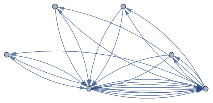
which can be more nicely visualized on the Poincaré disk using:
Each vertex corresponds to a maximally-symmetric Wyckoff position in the cell and its coset representatives (in Δ) can be accessed using:
which are given in terms of the translation generators:
This allows us to “unfold” or “flatten” the graph by displaying edges with an associated translation across copies of the cell (rather than inside a single cell):
Cell boundary
Cell boundary
For the compactification it is crucial to have access to the boundary of the cell, the identification of parts of the boundary with other parts, and the involved translations. This information is accessible as follows:
Faces
Faces
Finally, we also have access to oriented faces of the graph, which in the case of a cell graph are the quadrilaterals consisting of two mirror related Schwarz triangles making up the cell:
Due to the degeneracy of the graph, it is more instructive to consider the “flattened” versions:
Model graphs
Model graphs
So far, we have only worked with the cell graph, i.e., the nearest-neighbor graph of all maximally-symmetric Wyckoff positions. While it would be possible to define a tight-binding model directly on the cell, it is more convenient and efficient to let the HyperCells package handle part of it by first deriving a model graph.
We now have the relevant information for defining arbitrary tight-binding models on the chosen hyperbolic lattice. We simply need to place degrees of freedom at the vertices (potential with onsite potentials) and specify the coupling (hopping) between each pair connected by an edge. This results in a translation-invariant Hamiltonian of the form
While these quantities are constant in this case, generally, theey are functions of the vertices and edges (for the hoppings); we will discuss more general models demonstrating how that works further below.
Bloch Hamiltonian
Bloch Hamiltonian
Density of states
Density of states
For faster evaluation, we first compile the expression for the Bloch Hamiltonian:
The computation of the density of states (DOS) can take advantage of the independence of different momentum sectors and can therefore be parallelized:
dosT26 = ComputeDOS[cfHT26, 10^9, 32, {-8 - 0.005, 8}, 0.005];
Two nontrivial examples
Two nontrivial examples
In order to demonstrate how to define more complicated models, we consider two nontrivial examples.
Haldane model on the {8,3} lattice
The generalization [D. M. Urwyler, P. M. Lenggenhager, I. Boettcher, R. Thomale, T. Neupert, and T. Bzdušek, Hyperbolic topological band insulators, Phys. Rev. Lett. 129, 246402 (2022)] of the original Haldane model on the honeycomb lattice to hyperbolic lattices allows us to illustrate how to define a tight-binding model with multiple sites per unit cell, next-nearest-neighbor hopping amplitudes, as well as a site-dependent potential.
The model graph takes the following form:
To disentangle the hoppings, we can visualize nearest- and next-nearest-neighbor hoppings separately:
Since the graph contains information about which edges correspond to nearest neighbors and which to next-nearest-neighbors and the latter are already correctly oriented, the hoppings can be simply implemented as follows:
The A sublattice consists of the sites
such that the sublattice potential is
With this information, we construct the Abelian Bloch Hamiltonian on the primitive cell:
Click on the matrix to see high resolution version
Benalcazar-Bernevig-Hughes on the {6,4} lattice
Benalcazar-Bernevig-Hughes on the {6,4} lattice
With this information, we construct the Abelian Bloch Hamiltonian on the primitive cell:
Click on the matrix to see high resolution version
Supercell method
Supercell method
Underlying principles
Underlying principles
So far, we have focused on Abelian hyperbolic band theory, which relies on one-dimensional irreducible representations of the hyperbolic translation group. However, since hyperbolic translation groups are generally non-Abelian, i.e., noncommutative, there are higher-dimensional irreducible representations that contribute to the spectrum of the Hamiltonian. While the Bloch theorem extends to such states [J. Maciejko and S. Rayan, Automorphic Bloch theorems for hyperbolic lattices. Proc. Natl. Acad. Sci. U.S.A. 119, e2116869119 (2022)] and the definition of the associated Bloch Hamiltonian takes the same form,
where D is now a higher-dimensional irreducible representation of Γ, actual computations are complicated by missing parameterizations of such irreducible representations.
Extending models to supercells
Extending models to supercells
The first step in applying the supercell method to a given model such as the ones discussed above is to define the same model on larger supercells. The output provided by the HyperCells package together with the functionality of the HyperBloch package makes this process very easy. Conceptually, the supercell consists of translated copies of the primitive cell, such that extending a model defined on the primitive cell amounts to identifying the preimage (in the primitive cell) of each site or bond in the supercell under the appropriate translation and simply assigning the same values for onsite potential and hopping as in the primitive cell.
which we can import using:
This returns an object with head HCSupercellModelGraph containing the relevant information about the supercell and its relation to the primitive cell. For example, the embedding homomorphism of the supercell translation group into its supergroup, the primitive-cell translation group:
Crucially, all vertices and edges in the supercell graph refer back to their preimage in the primitive cell and provide information about the relevant translation. For vertices, the first two elements give the label of the corresponding vertex in the primitive cell (here both are translated copies of the single vertex {3,1}):
while the third element gives the index in the list of supercell-internal translations:
To visualize the supercell boundary, we also need to import the information about the compactification of the supercell:
Then, we can show the supercell model graph on the supercell:
Similarly, the edges contain information about the preimage of each vertex (the first and second element of the edge tag give the index of the vertex in the list of vertices in their corresponding copies of the primitive cell, here 1 for both) and the tag of the preimage of the edge (third element of the tag; this matches uniquely with one edge in the model on the primitive cell):
Under the hood, this allows the HyperBloch package to assign onsite potentials and hopping amplitudes in the full supercell with them only explicitly defined on the primitive cell:
Note that we have provided the exact same input as for the model on the primitive cell with the only two differences being: (1) the first argument is an HCSupercellModelGraph object instead of an HCModelGraph and (2) we provided the corresponding HCModelGraph describing the model on the primitive cell as an option PCModel.
While the present model is simple enough to be easily defined directly on a supercell, the advantages of this method become clear to a more complicated model such as the Haldane or BBH model introduced above.
Application: converging density of states
Application: converging density of states
With the model defined on a supercell, we can now easily evaluate and diagonalize the Abelian Bloch Hamiltonian on that supercell, which will, effectively, provide us with non-Abelian states on the primitive cell in addition to the Abelian ones. This explains the very drastic change in the density of states:
dosT311 = ComputeDOS[cfHT311, 10^9, 32, {-8 - 0.005, 8}, 0.005];
Crucially, the density of states converges eventually when going to larger supercells. Here we simply show data taken from https://doi.org/10.5281/zenodo.10142168 and do not repeat the resource-intensive calculations (but the procedure is identical to the above, just with different supercells):
Convergence with number of randomly sampled momenta
Convergence with number of randomly sampled momenta
Comparison to results obtained on PBC clusters
Comparison to results obtained on PBC clusters
This should be contrasted with the results obtained on finite clusters with periodic boundary conditions (of the same size as the supercell but without introducing momenta):
Comparison of different sequences of supercells
Comparison of different sequences of supercells
Alternative sequences give rise to compatible results:
Haldane model on the {8,3} lattice
Haldane model on the {8,3} lattice
While convergence of the supercell method can already be observed by studying the elementary nearest-neighbor model on the {8,8} lattice (surprisingly reasonable results are obtained already on supercells with only 64 sites), we briefly consider the result of applying the supercell method to the Haldane model on the {8,3} lattice.
Due to the larger number of sites per unit cell, namely 16, convergence is much faster, both in number of momenta and in supercell size. In particular, we can here already obtain a reasonably converged density of states from sampling just 1000 momenta:
Increasing the momentum sampling still improves the density of states, but only marginally and without any qualitative changes:
Conclusion
Conclusion
The supercell method introduced in the original research article together with the HyperCells and HyperBloch packages provide an easy method for studying non-Abelian Bloch states for arbitrary tight-binding models defined on hyperbolic lattices. Besides enabling the user to easily define and study tight-binding models, the visualization functions provided by the HyperBloch package help with designing models and translating between the algebraic description of hyperbolic lattices in terms of triangle groups and their geometric representation in the Poincaré disk.
We anticipate the supercell method and the publicly available software packages to facilitate advances in the study of hyperbolic lattices, such as in symmetry analysis, low-energy expansions, and topological band theory.
CITE THIS NOTEBOOK
CITE THIS NOTEBOOK
Non-Abelian hyperbolic band theory from supercells
by Patrick M. Lenggenhager, Joseph Maciejko and Tomáš Bzdušek
Wolfram Community, STAFF PICKS, February 27, 2024
https://community.wolfram.com/groups/-/m/t/3131734
by Patrick M. Lenggenhager, Joseph Maciejko and Tomáš Bzdušek
Wolfram Community, STAFF PICKS, February 27, 2024
https://community.wolfram.com/groups/-/m/t/3131734