ORIGINAL ARTICLE: Zhaobin Xu, Jian Song, Hongmei Zhang, Zhenlin Wei, Dongqing Wei, Jacques Demongeot, A Mathematical Model Simulating the Adaptive Immune Response in Various Vaccines and Vaccination Strategies, medRxiv 2023.10.05.23296578. DOI: https://doi.org/10.1101/2023.10.05.23296578
Introduction:
Introduction:
The accomplishments of vaccination are undeniable, leading to significant advances in human health. Yet, new infectious diseases and evolving pathogens constantly challenge our understanding of vaccine efficacy and immunity. Mathematical modelling is a crucial lens through which we can reach a more comprehensive understanding of these complexities. By simulating the biological responses to vaccines, models can provide critical insights into disease progression, vaccine performance, and optimal strategies for developing vaccines.
In this short text, we’ll explore an approach to constructing one such model in the Wolfram Language. We will reproduce a compartmental dynamical model of adaptive immune responses to vaccine treatments described in a recent preprint from medRxiv.org: A Mathematical Model Simulating the Adaptive Immune Response in Various Vaccines and Vaccination Strategies (Xu et al. 2023). Compartmental models are a class of mathematical models which divide variables of interest into sections or “compartments”. Each compartment represents a specific state within the system being studied. The models track how entities, like cells or molecules, interact within and between these compartments over time.
The stated goal of the paper is to construct a novel mathematical model to quantitatively research the activation of adaptive immune responses by vaccines. This model is used to simulate and compare the dynamics of antibody levels after administering different types of vaccines (inactivated, attenuated live virus, mRNA), thereby contributing to a better understanding of the mechanisms of various vaccines and vaccination strategies. Through the model, the authors aim to suggest strategies for vaccine design, while providing a comprehensive portrait of the inducible interactions between antibodies and antigens in the immune process.
Setup
Setup
Dependencies
Dependencies
In[]:=
PacletInstall["RobertNachbar/CompartmentalModeling"]
Out[]=
PacletObject

In[]:=
Needs["RobertNachbar`CompartmentalModeling`"];
Paper Tables
Paper Tables
Reactions, Parameters, and State Variables of the Model
Reactions, Parameters, and State Variables of the Model
The authors of the paper helpfully provide three tables fully specifying the interactions between state variables (components) of the system, as well as model parameters and initial conditions. I have reproduced these tables below. Note that some parameter values and initial conditions depend on the selected vaccine treatment type. More precisely:
◼
The replication rate of viral antigens, described by parameter should be set to in the case of a simulation of the administration of an attenuated live virus vaccine, and 0 otherwise.
k
14
.3
◼
The initial condition of the state variable , (Antigen) should be set to for simulation with an inactivated vaccine, 0 with an mRNA vaccine, and 1 for an attenuated live virus vaccine.
x
2
6
10
◼
The initial condition of the state variable , (mRNA) should be set to 0 for simulation with an inactivated or attenuated live virus vaccine, and for and mRNA vaccine.
x
9
6
10
For a more in depth explanation of these parameters and initial conditions, please refer to the paper.
Table 1: Model reaction index and descriptions.
Out[]=
Table 2: Estimates of the model parameters.
Out[]=


Table 3: Time-dependent variables of the model characterizing the antibody-antigen interactions
Out[]=
Extracting Model Information
Extracting Model Information
We can use tools from the CompartmentalModelling paclet to extract useful information about the model. For instance, we can use CompartmentalModelGraph from the CompartmentalModel paclet to visualise the model’s structure:
CompartmentalModelGraph[reactions["Reaction"],ImageSize->Full]
Out[]=
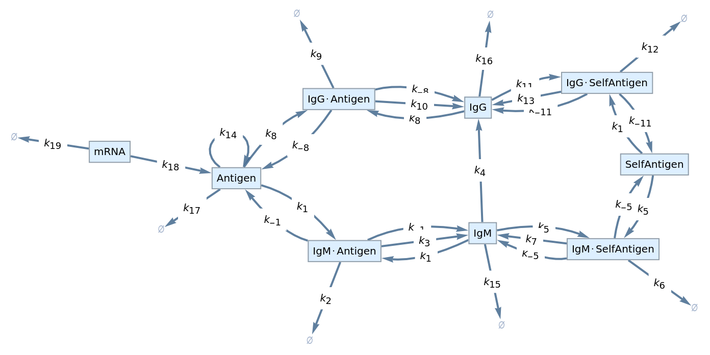
The CompartmentalModelling paclet contains convenient functions to streamline the process of building models. For instance, we can use KineticCompartmentalModel to generate differential equations for from a list of component transitions (the reactions).
Fetch model data:
modelData=KineticCompartmentalModel[reactions["Reaction"],t];Dataset[modelData]
Out[]=
These data are very useful for quickly building and simulating compartmental models.
Numerical Simulations
Numerical Simulations
Preparing Model ODEs
Preparing Model ODEs
Owing to details related to the original code implementation of the model, the authors provide a slightly modified system of ODEs describing the model. This system is reproduced below and numerically approximated using NDSolve for different vaccine treatments:
Reproduce the system of ODEs from the paper:
Let’s also get some replacement rules to easily convert between the variable names in plain English, and the symbols used in the paper for the model’s system of ODEs.
Plain English variables ODE variables:
Vaccine Treatment Simulations
Vaccine Treatment Simulations
In the paper, the authors model three cases:
1
.Inactivated Vaccine Simulation.
2
.Attenuated Live Virus Vaccine.
3
.mRNA Vaccine
1. Inactivated Vaccine Simulation
1. Inactivated Vaccine Simulation
Model-specific parameters and initial conditions:
Define model parameters corresponding to the inactivated vaccine setup:
Define initial conditions of the system corresponding to the inactivated vaccine setup:
Construct the system of equations for NDSolve, with parameter values and initial conditions:
Plot the solution:
2. Attenuated Live Virus Vaccine
2. Attenuated Live Virus Vaccine
Model-specific parameters and initial conditions:
Define model parameters corresponding to the attenuated live virus vaccine setup:
Define initial conditions of the system corresponding to the attenuated live virus vaccine setup:
Construct the system of equations for NDSolve, with parameter values and initial conditions:
Solve numerically with NDSolve:
Plot the solution:
3. mRNA Vaccine
3. mRNA Vaccine
Model-specific parameters and initial conditions:
Define model parameters corresponding to the mRNA vaccine setup:
Define initial conditions of the system corresponding to the mRNA vaccine setup:
Construct the system of equations for NDSolve, with parameter values and initial conditions:
Plot the solution:
Closing notes
Closing notes
Through the exploration of this dynamical immune response model, we have seen how mathematical modelling in the Wolfram Language, can be used to derive insights into complex biological systems.
If you are interested in this work, and would like to learn more, please make sure to give the source paper a read! This post is primarily designed to demonstrate how one might conduct this form of modelling in the Wolfram Language. I also highly encourage you to try Bob Nachbar’s CompartmentalModelling paclet. The CompartmentalModelling paclet is not just for biologists, but could be a valuable tool for anyone dealing with interconnected systems that can be represented as compartments. As always, I welcome your notes and comments! Please do not hesitate to reach out to me! I look forward to your thoughts!
CITE THIS NOTEBOOK
CITE THIS NOTEBOOK
A dynamical model of immune-system response to mRNA, live virus, and inactivated vaccines
by Phileas Dazeley-Gaist
Wolfram Community, STAFF PICKS, October 25, 2023
https://community.wolfram.com/groups/-/m/t/3055726
by Phileas Dazeley-Gaist
Wolfram Community, STAFF PICKS, October 25, 2023
https://community.wolfram.com/groups/-/m/t/3055726