A Turing machine is a theoretical model of computation classified as an automaton invented by Alan Turing that operates on an infinite tape of sequential memory. The significance of Turing machines, as described in the Church-Turing thesis, comes from their ability to compute any function and therefore have the same computational ability as all conventional computers. Empirical evidence suggests that there exists Turing machines that follow different rules but ultimately compute the same function, presumably for all inputs. Naturally, these machines will have different runtimes, which models multiple computers running different algorithms to reach the same goal. Similarly, motivation for studying complexity theory comes from analyzing and improving algorithms. A central unsolved problem in the field is if quickly verifying a solution to a problem implies the existence of an algorithm that quickly solves it—commonly known as the P vs. NP problem. Analyzing patterns in the range of runtimes for equivalent Turing machines provides potential for empirically hypothesizing at the relationship between P and NP.
Introduction
Introduction
Formally, a Turing machine is a tuple of a set of states, a halt state, a set of symbols called its alphabet, and a lookup table of all possible state-symbol pairs. Turing machines keep a pointer to the cell it is currently reading, and the symbol on this cell combined with its current state defines a transition. For each transition, three operations occur: read the symbol on the current cell, write a (not necessarily distinct) symbol to the current cell, and move to an adjacent cell. Certain traits of a Turing machine are difficult to quickly represent with a real computer, so the results in this essay will be close approximations of the real behavior of Turing machines. Specifically, we will bound a finite section of the tape and set a halting condition as when the head moves left of its starting point used in S. Wolfram, A New Kind of Science. Wolfram Media, 2002 instead of the orthodox method of having a halting state.
Terminology
Terminology
In this essay, the variables and generally refer to the states and symbols of a Turing machine, and the ordered pair refers to an -state -symbol Turing machine. Additionally, we define setting a Turing machine to a nonnegative integer as filling our chosen interval of the tape of length for some with the binary representation of in big endian (natural left-to-right order). We ensure that the number of bits fits in (i.e. ). Additionally, we define the value of a Turing machine as the number created by each cell on as base- digits where the blank symbol translates to zero. Later, we propose a slightly different way of interpreting the value.
s
k
s
k
(s,k)
s
k
x
I
W
W
x
W
⌊(x+1)⌋≤W
log
2
I
k
Formalism
Formalism
Let be the set of all -state -symbol Turing machines. Each machine in represents a partial function ⇀ on a fixed interval of length on the tape where is the set of symbols and is the set of input symbols. For this essay, we set . Equivalently, this function can also be represented as ⇀ with input specified by the base number formed on where each symbol is an integer between 0 and . Define two Turing machines in to be equivalent if they compute the same partial function on , or both do not exist. The number of distinct machines is then the cardinality of . For each equivalence class, we will analyze patterns of the worst-case running times of each machine in the class and over all classes in for different and .
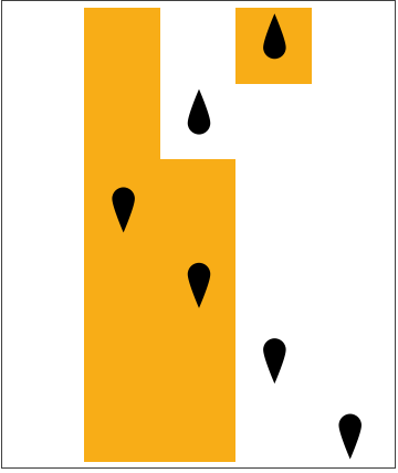
For example, the following 2-state 2-symbol Turing machine takes in where 1’s are colored orange. The output is read as 6. It turns out that this rule always adds 1 to the input for our constraints.
T
sk
s
k
T
sk
f:
w
Σ
w
Γ
I
w
Γ
Σ⊆Γ
ΣΓ
f:
k
I
k-1
T
sk
I
T
sk
T
sk
s
k
For example, the following 2-state 2-symbol Turing machine takes in
5
0101
2
0110
2
Evolution of the function described by rule 451 for , input for 5 steps:
f(x)x+1
(n,k)(2,2)
x5
Out[]=
Theory
Theory
Only certain pairs are capable of simulating any other Turing machine starting from a blank tape. For example, any Turing machine with one symbol trivially fails to be universal because it will not edit the tape. Pairs that can simulate all other machines are known as universal Turing machines. Additionally, weakly universal Turing machines are machines that are universal on an arbitrary initial tape. Notably, the smallest of these machines are fully analyzable within computational constraints, such as , , and Wolfram’s machine.
The universality of Turing machines as a mathematical model of computation revealed limits of computing, notably cases of logical (un)decidability. A problem is undecidable if and only if it is provable that there exists no algorithm that will always return the correct answer to the problem. Turing’s major result was his proof of the undecidability of determining if a computer program halts, famously known as the halting problem.
(n,k)
(3,3)
(2,4)
(2,3)
The universality of Turing machines as a mathematical model of computation revealed limits of computing, notably cases of logical (un)decidability. A problem is undecidable if and only if it is provable that there exists no algorithm that will always return the correct answer to the problem. Turing’s major result was his proof of the undecidability of determining if a computer program halts, famously known as the halting problem.
The Halting Problem and Rice’s Theorem
The Halting Problem and Rice’s Theorem
The usefulness of the undecidability of the halting problem is not only limited to the statement itself, but because many problems can be shown to be undecidable by reducing them to the halting problem. More notably, it is undecidable to determine if two Turing machines are equivalent, which necessitates the mentioned constraints. Similarly, the task to quickly analyze the behavior of a Turing machine without simulating it is a generalization of the halting problem known as Rice’s theorem, which implies that this task is generally undecidable. However, it does not say anything about determining relationships between machines, which we will see in a later section could contain a predictable pattern.
Implementation
Implementation
Due to the undecidability of universal static analysis and the computational irreducibility of Turing machine evolution, the implementation will inevitably be brute-force in nature. However, there are certain ways to prune the search space by examining only the rules. There are also optimizations for Turing machine simulation, particularly with memoizing sections of the tape.
Prune
Prune
Despite the undecidability of finding a universal way of reducing computation across Turing machines or even on one Turing machine, we can take inspiration from DFA (deterministic finite automaton) minimization. Specifically, one big optimization we can make is to declare that all Turing machines with rules that permute a dead state (unreachable from the initial state) to be equal: each of these permutations are unreachable anyway.
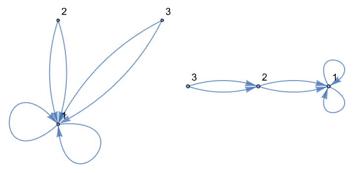
The diagram below shows two equivalent Turing machines, each with a different permutation of the rules from state 2, which is unreachable from state 1.
The diagram below shows two equivalent Turing machines, each with a different permutation of the rules from state 2, which is unreachable from state 1.
Out[]=
Determining the reachable nodes reduces to graph traversal. It is not hard to see that all state graphs have vertices and edges, resulting in a runtime of . Building this graph is straightforward by simply inspecting the full form of the Turing machine rule.There are two ways to describe a Turing machine rule in the Wolfram Language: full form as a list of transitions, or an index as an integer. We want to take advantage of the language’s indexing method to skip over redundant rules. Increasing the index permutes rules in the following order: direction (-1 to 1), then symbol (0 to ), then state (1 to ). Notice that if the reachable states are consecutive (which must include state 1), we can permute the rest of the states that are unreachable without changing what the TM does. For example, a 3-state TM can only reach states 1 and 2, we can permute the rules from state 3, which defines a contiguous interval of rule numbers that are equivalent (i.e. rules 83520 to 84096 for a (3,2) TM). Thus, for each of these intervals we see, we can skip ahead to the end of the interval when we detect a beginning to avoid checking redundant rules.The length of an iteration depends on the number of reachable states. If there are reachable states from 1 to , then there are unreachable states. The number of ways we can permute these unreachable states is given by , since there are symbols per state and ways to permute each single component of a rule. Notice is the number of s-state k-symbol Turing machines.
n
nk
O(n(k+1))
k-1
n
d
d
n-d
P(d)
k(n-d)
(2nk)
k
2nk
P(0)
Returns :
P(d)
In[]:=
perm=Function[{d,s,k},(2sk)^(k(s-d))];
There exists resource functions for converting between the two forms of a Turing machine rule, but as we will see later, these functions are too slow, so I have taken their source code and written a compiled version. We will also declare in our environment so it can be used in compiled functions.
perm
Reset the compiler environment:
In[]:=
$CompilerEnvironment=CreateCompilerEnvironment[];
Compiled TuringMachineFromNumber and TuringMachineToNumber
Compiled TuringMachineFromNumber and TuringMachineToNumber
Compiled Graph Build and DFS
Compiled Graph Build and DFS
Compiled Transform and Other Functions
Compiled Transform and Other Functions
Pruning
Pruning
The following function determines the number of unique rules and the number of times each rule is repeated. To dynamically skip blocks of rules as outlined previously, we must use a loop to have full control over the index. To determine if the current rule is the start of a block, we do a graph traversal in time, which is done times.
For
Θ(sk)
O
sk
(2sk)
Takes in the number of rules to analyze from 0 to and loops through those rules, skipping if possible:
len-1
In[]:=
cfprune=FunctionCompile[Function[{Typed[len,"MachineInteger"],Typed[s,"MachineInteger"],Typed[k,"MachineInteger"]},Module[{i,map=CreateDataStructure["HashTable"]},For[i=0,i<len,i++,With[{rule=cfTuringMachineFromNumberCompiled[i,s,k]},With[{vout=Cast[cfdfs[cfadjinit[s,Module[{a=CreateDataStructure["FixedArray",sk]},Do[a["Part",i]=First[rule[[i]]][[1]]->Last[rule[[i]]][[1]],{i,sk}];a["Elements"]](*returnsrule[[All,All,1]]*)],1,s],"PackedArray"::["MachineInteger",1]]},map["Insert",(#->If[cfconsQ[Sort[vout]],(i+=#-1;#)&@cfperm[Length[vout],s,k],1]+If[map["KeyExistsQ",#],map["Lookup",#],0])&@cfTuringMachineToNumberCompiled[With[{left=Transpose[{Flatten[Table[ConstantArray[j,k],{j,s}]],Table[Mod[j,k],{j,sk-1,0,-1}]}],right=cftransform[s,k,vout,Cast[Last/@rule,"PackedArray"::["MachineInteger",2]]]},Module[{a=CreateDataStructure["FixedArray",sk]},Do[a["Part",i]=left[[i]]->right[[i]],{i,sk}];a["Elements"]]],s,k]];]]];map["Elements"]]]];
Get elements for (2,2) TM’s:
In[]:=
elems=cfprune[perm[0,2,2],2,2];
Get elements for (3,2) TM’s (this takes a while):
elems23=cfprune[perm[0,3,2],3,2];
We can confirm that consecutive equivalence classes come in sizes of for all . In this case, for , we indeed have 1 and 1728. For (3,2), we will have 1, 144, 20736.
ki
(2nk)
0≤i<n
(s,k)(2,3)
0
12
3
12
0
12
2
12
4
12
DeleteDuplicates[elems32[[All,2]]]
Out[]=
{1,144,20736}
Search
Search
As mentioned, the behavior of a Turing machine is undecidable even on a finite tape, so we must optimize our simulation method. One notable bottleneck—amongst others—is repeating and non-terminating Turing machines. Optimizing repeating machines can be “solved” by memoizing a “snapshot” of the Turing machine for each independent round of simulation of a machine and an input, and after each iteration, we check if the current snapshot has been seen before. However, this “solution” does not address the main bottleneck of the program, which is that it has to construct the TM tape for each step in its iteration, which is an operation. Therefore, I have written a compiled version of the TuringMachine function that only returns the part of the tape we want after the TM halts.
O()
2
n
Compiled TM function that returns a pair of :
{{a1,a2,...},{runtime}}
Call function in parallel. Wolfram internal parallelization functions should preserve order:
Get compressed file of the halting configuration of (2,3) TM’s and copy it locally:
Load the file once it is decompressed:
In this scheme, there are 748 (2,2) TM’s that do not halt, and there 353 different functions that can be computed. Stephen Wolfram in NKS found there to be 351 different TM’s, which may be caused by a slight difference in constraints and setup.
Gather (2,3) TM’s:
For (2,3) TM’s, there are 225,263 machines that don’t halt and 448,335 different functions:
Gather (3,2) TM’s:
For (3,2) TM’s, there are 435,012 machines that don’t halt and 43,676 different functions:
Runtime Distribution Analysis
Runtime Distribution Analysis
In this section, we visualize our computed results and draw attention to global relationships between each computed function and their runtimes. Note that all data fetched from the cloud were computed using the code in the previous section.
Plots
Plots
On the plots below, the top plot shows the size of the equivalence class, or the number of TM’s that compute the function; the middle plot shows the runtime range; the bottom plot shows the minimum and maximum runtime for a function. Notice that runtime range decays very quickly and the minimum and maximum runtime consequently converge quickly. It is worthy of stating that for the Turing machine analog of complexity classes, a function is classified based on its minimum runtime. The functions of interest are ones with a low minimum runtime but high maximum runtime and thus high runtime range, which represent problems that seem to be NP-hard but can be solved in P. These functions occur at the very beginning of the plot where the runtime range is high. Consequently, the second type of function we are interested in are ones that behave truly NP: that is, they have a high minimum runtime, which usually means low runtime range. These functions can be seen sparsely on the plot below from 240 to 250 and from 290 to 300.
Get and plot (2,2) data:
Plot the first 2000 and last 5000 groups of (2,3) TM data sorted by runtime range side by side:
Plot the first 2000 and last 5000 groups of (3,2) TM data sorted by runtime range side by side:
Generates (2,4) plot for the random size 2 million subset:
If we observe the plots for (2,4), (4,2) and (3,3) TM’s, we notice that the shape of the decay rates indeed stay similar and the spikes at the end are still there despite being slightly messier. Calculating the proportion for these three (s,k) combinations, we get
(2,4):
(4,2):
(3,3):
Rule Distribution
Rule Distribution
We notice that many equivalence classes contain consecutive blocks of rules of the same size—which do not contain the blocks we pruned out. Additionally, there are many pseudo-connected rules belonging to the same equivalence class with small gaps between them, such as the blue and yellow lines near the beginning, which suggests that predictable and consistent pruning can be done in “neighborhoods” of rules. Non-consecutive blobs of rules that have unreachable states in their state graph form an arithmetic sequence and would have regularity on the graphic, but the intriguing part is that cases of unreachable states are relatively uncommon, yet for almost all equivalence classes shown, there is some form of regularity.
Runtime Analysis
Runtime Analysis
Note
Note
Generates a list of runtime plots from a list of rule numbers:
(2,2) TM’s
(2,2) TM’s
Get sorted equivalence classes by runtime range:
The following graphics depict the runtime plot of a TM with a certain rule number for each group sorted by runtime range. In each plot, the runtime for the TM is plotted against the value of the input on the tape. The plots are ordered from largest max runtime to smallest max runtime.
Runtime plots for the first group sorted by runtime range (the group with the largest runtime range):
Notice how the runtime for rules 378 increases asymptotically linearly but at some spots have much shorter runtimes. Rule 1409 increases approximately logarithmically also with gaps, and rule 3919 runs in constant time. As a sanity check, these plots agree with what we see if we simulate each of these rules on a TM with the number 3 in binary on the tape.
This is an example of where the dominating linear TM (378) can be improved significantly (since this function simply does nothing so there exists a TM that solves it in constant time).
Merged runtime plot showing the worse case linear growth rate:
Another group worth pointing out is the 15th function shown below, where there are TM’s that grow linearly and logarithmically, which is another example of where a function’s runtime can be improved, but non-trivially. However, most of the first 40 functions are simply computed by TM’s with the same asymptotic runtime but at different magnitudes, which I hypothesize means that for non-trivial functions, most improvements are going to be reductions by a constant factor instead of in growth rate.
Separate runtime plots for select TM’s in the 4th function:
We can also sort by maximum runtime:
Generates plots for the first 36 groups sorted by maximum runtime:
If we generate the separated plots for the first 36 functions (with the function above), observe that most of these functions are only computed by a single or a few TM’s, which may represent problems that are intrinsically difficult to even find a solution for. However, the 29th and 36th functions are interesting in that both are computed by 9 different TM’s, and all of those run in logarithmic time, which represents a more non-trivial function where there are many known solutions but none of them are trivially fast. Strangely, both of these functions trace the same graph...
Runtime plot for the 29th and 36th function, respectively:
Plotting by length, we indeed see that the linear function becomes exponential and the logarithm becomes linear. Similarly, taking the average of runtimes for a given length will result in an approximately linear and logarithmic graph like the uncompressed visualization.
(2,3) TM’s
(2,3) TM’s
We do the same for the (2,3) data:
Plot certain runtimes for the function with the largest runtime range:
Notice that the first two runtimes unsurprisingly grow exponentially but there also exists a TM that grows linearly without a large constant factor. Fitting the data into an exponential, we get the following equation and R-squared value. This is an elegant example of a problem in P where exponential solutions can be improved to linear.
Fit and R-squared for an exponential:
The anticipated runtimes for an NP-hard function would be where most Turing machines that compute the function compute it near the maximum runtime of all TM’s. This is the opposite of the P problem shown above where there are TM’s that have a high maximum runtime but others with a low maximum runtime. In the (2,3) plot and with the code below, we see that runtime range decreases very quickly, meaning there are a pretty small number of relevant P problems with non-optimal solutions. Below calculates the ratio between the number of P and NP behavior problems:
Gets the number of functions with runtime range ≥400 and the number of functions with min runtime ≥400:
The second being greater than the first means that there are more problems that seem to be NP-hard and cannot be improved than problems in P that have superpolynomial algorithms that can be optimized/modified. Since these numbers are very small relative to the 448,334 functions in (2,3) space, I hypothesize means that we need more states and symbols to have a large enough search space to properly represent non-trivial functions, which will be essentially computationally infeasible for exhaustive search.
One last manipulation we can do is to sort the compressed data (by max runtime) by how rapidly they increase. I claim that the following function is a sufficient heuristic for this sort.
One last manipulation we can do is to sort the compressed data (by max runtime) by how rapidly they increase. I claim that the following function is a sufficient heuristic for this sort.
Group (2,3) TM functions and add a growth rate heuristic:
By inspection, exponential growth rate tends to collapse at around the 800th function (which is not a lot considering there are 448334 functions in total), so we sample the first 800 functions and count the ones with small runtime range as NP behavior (≤20 in this case) to get a proportion between functions with P behavior and NP behavior.
The above proportion is not too far off the proportion found with runtime range and max runtime (0.237), which suggests that for the TM analog of complexity classes, there are classes harder than P that cannot be reduced to P and have substantially more problems in them (can we say about 5 times more?).
(3,2) TM’s
(3,2) TM’s
We will do something very similar to (2,3) TM’s.
Sort data:
Plot select TM’s from the function with the largest runtime range:
When we look for the proportion of functions with P and NP behavior, we reduce the range threshold to 250 because the maximum runtimes and thus runtime ranges for (3,2) TM’s are smaller (there are only 2 functions with runtime range ≥400), and the (3,2) graph in the previous section also decayed faster.
Number of functions with runtime range ≥250 and number of functions with min ≥250:
Notice how this 0.196 ratio is similar to the (2,3) proportion of 0.237 which serves as more evidence that there are more NP-hard problems that cannot be improved than ones that can. Finally, we can sort by growth rate again to find a more accurate proportion.
Group (3,2) TM functions and add a growth rate heuristic:
This time exponential growth rate tends to already collapse at around the 40th function (compared to the 800 for (2,3) TM’s), so we sample only the first 40 functions and count the ones with small runtime range as NP behavior (again with 20 as the range threshold).
Larger (s,k) TM’s
Larger (s,k) TM’s
This data was ran without storing the rules since we did not do any pruning and can simply treat the index as the rule number. We begin by analyzing (2,4) and directly adding the growth rate heuristic.
(2,4)
(2,4)
Gather the subset of (4,2) TM’s:
At this point, we will skip the plots and directly calculate the P and ≥NP proportions:
As predicted, this ratio is again smaller.
(4,2)
(4,2)
For (4,2), we have
Calculate the first proportion:
Surprisingly, this number is even higher than the first proportions of (2,3) and (3,2), and I have yet to figure out why this is. Moving to the second proportion with a threshold at 20 (again, by inspection), we have
which is an even higher ratio than before.
(3,3)
(3,3)
Finally, for (3,3), we have
Calculate the first proportion:
The growth rates for (3,3) are less clean and it becomes ambiguous where to place a threshold, so we will use 200 as an approximation.
Calculate the second proportion:
Summary of Conclusions
Summary of Conclusions
Without doing any calculation, inspecting the plots of the first 5 functions with exponential runtime suggests that there are no problems in the (2,2) space with NP behavior, since the exponential TM’s can be improved to constant or linear time.
Generate the longest and shortest runtime plots for the first 5 functions:
Future Directions
Future Directions
◼
Further analyze the TM runtimes and use different runtime schemes to find more general patterns not specific to a single runtime scheme
◼
Optimize current implementations and add more advanced optimization
◼
Investigate the ratio increase of (4,2) TM’s
◼
Extend to nondeterministic Turing machines to try to resolve the issue brought up in the previous section of not knowing the relative cardinality of P, NP, EXPTIME, etc.
Acknowledgements
Acknowledgements
I would like to thank my mentor Felipe Amorim for supporting me throughout this project, keeping me on track, and helping me organize and implement my ideas. I would also like to thank my teaching assistant Gregory Roudenko for inspiring the methods I used for code optimization, mentor Shenghui Yang for explaining code compilation and approaches to code optimization, and the program directors Rory Foulger, Megan Davis, and Eryn Gillam for accepting me into WSRP. Finally, I would like to thank Dr. Stephen Wolfram for giving me this illuminating project and its motivation as an unconventional approach to complexity theory.
References
References
1
.Ariel (https://cs.stackexchange.com/users/27055/ariel), Given two total Turing machines, is it undecidable problem to detect whether they give the same output on all inputs?, URL (version: 2015-08-30): https://cs.stackexchange.com/q/45687
2
.Manlio (https://math.stackexchange.com/users/22701/manlio), How are weakly universal Turing machines actually defined?, URL (version: 2020-04-22): https://math.stackexchange.com/q/3634837
3
.Weisstein, Eric W. “Turing Machine.” From MathWorld--A Wolfram Resource. https://mathworld.wolfram.com/TuringMachine.html
4
.Wikipedia contributors. (2025, June 30). Automata theory. In Wikipedia, The Free Encyclopedia. Retrieved 15:56, July 9, 2025, from https://en.wikipedia.org/w/index.php?title=Automata_theory&oldid=1298074772
5
.Wikipedia contributors. (2025, April 14). DFA minimization. In Wikipedia, The Free Encyclopedia. Retrieved 15:59, July 9, 2025, from https://en.wikipedia.org/w/index.php?title=DFA_minimization&oldid=1285525404
6
.Wikipedia contributors. (2025, June 12). Halting problem. In Wikipedia, The Free Encyclopedia. Retrieved 21:23, July 9, 2025, from https://en.wikipedia.org/w/index.php?title=Halting_problem&oldid=1295203495
7
.Wikipedia contributors. (2025, March 18). Rice’s theorem. In Wikipedia, The Free Encyclopedia. Retrieved 15:58, July 9, 2025, from https://en.wikipedia.org/w/index.php?title=Rice%27s_theorem&oldid=1281112418
8
.Wikipedia contributors. (2025, June 24). Turing machine. In Wikipedia, The Free Encyclopedia. Retrieved July 2, 2025, from https://en.wikipedia.org/w/index.php?title=Turing_machine&oldid=1297184647
9
.Wikipedia contributors. (2025, March 17). Universal Turing machine. In Wikipedia, The Free Encyclopedia. Retrieved 15:55, July 9, 2025, from https://en.wikipedia.org/w/index.php?title=Universal_Turing_machine&oldid=1281033475
10
.Wolfram, S. (2002). A New Kind of Science. Retrieved from https://www.wolframscience.com
CITE THIS NOTEBOOK
CITE THIS NOTEBOOK
Empirical analysis of P vs. NP: on the equivalence of Turing machines as partial functions
by Michael Sun
Wolfram Community, STAFF PICKS, July 10, 2025
https://community.wolfram.com/groups/-/m/t/3501455
by Michael Sun
Wolfram Community, STAFF PICKS, July 10, 2025
https://community.wolfram.com/groups/-/m/t/3501455