Variational Quantum Linear Solver
Variational Quantum Linear Solver
Theory
Theory
The Variational Quantum Linear Solver (VQLS) is a a hybrid quantum-classical technique designed to address the Quantum Linear Systems Problem (QLSP). It aims to find linear system solutions using quantum computing techniques.
The classical problem is formulated as follows:
Given a matrix A and vector b, find x such that
A.x=b
The corresponding quantum algorithm can be summarized as follows:
Given:
◼
Problem vector: A quantum state such that
|b〉
|b〉=U|0〉
◼
Problem matrix: × dimensional matrix such that , where ϵ and are unitary gates
n
2
n
2
A
A=
L-1
∑
0
c
l
A
l
c
l
A
l
We want to prepare:
◼
A quantum state such that and ->|b〉
|x〉
|ψ〉=A|x〉
|ψ〉
ψ
ψ
Precedents
Precedents
We have this relevant first implementation of a variational quantum circuit that solves linear systems by Bravo-Prieto, you can check the paper in the following link.
Bravo-Prieto VQLS
Bravo-Prieto VQLS
◼
First implementation of a variational quantum circuit for solving linear systems
◼
Requires multiple circuits (:
Gatesandpermute
A
i
CZ
j
◼
In general the algorithm performs the calculation in a real quantum computer by obtaining multiple expected values from multiple circuit variations.
◼
he diagram displayed is an example from one of those circuits, Gate A and the Control Z gate permute between different qubits to obtain the different expected values:
Out[]=

◼
He also used a local cost function in order to avoid getting stuck in local minimum values:
C
L
1
2
1
2n
n-1
∑
j=0
∑
l,l'
c
l
*
c
l'
μ
l,l',j
∑
l,l'
c
l
*
c
l'
μ
l,l',-1
where =〈0|UV|0〉, -> and ->0<->->0.
μ
l,l',j
†
V
†
A
l'
Z
J
†
U
A
l
Z
-1
C
G
C
L
You can check more about this implementation on my community post: https://community.wolfram.com/groups/-/m/t/3180154
Multiplexer-based VQLS
Multiplexer-based VQLS
We propose a Multiplexer–Based Variational Quantum Linear Solver (MB-VQLS). The primary distinctions between MB–VQLS and a conventional VQLS lie in two key aspects:
◼
The controlled implementation of the matrix through a multiplexer
A
◼
Quantum fidelity cost function:
f(ω)=1-
b
ψ(ω)
2
◼
The solution to the linear system is encoded directly in the amplitudes of the resultant quantum state.
Further steps will show that we can avoid some and restrictions using their normalization terms. This would help us find solutions for any system.
|b〉
A
A.x Operation Circuit Representation
A.x
Considering an × A matrix and an -element vector , we look to compute the operation with a quantum circuit using as a controlled operation.
n
n
n
x
A.x
A
To start, let’s define a complex vector x using RandomComplex, and a random real matrix A called “a”:
In[]:=
x=RandomComplex[{-1-1*I,+1+1*I},4]
Out[]=
{-0.126112-0.770322,0.302431-0.0695352,0.0386691-0.00105955,0.0950529-0.0692226}
We will begin the implementation by encoding the matrix A into the quantum circuit:
In[]:=
a=RandomReal[{-1,1},{4,4}];a//MatrixForm
Out[]//MatrixForm=
0.25529 | 0.831537 | 0.774413 | 0.967247 |
0.345805 | 0.29044 | 0.424374 | -0.428653 |
-0.406224 | 0.260866 | -0.687513 | 0.829075 |
-0.901911 | 0.438124 | -0.841926 | -0.108815 |
We proceed to generate a quantum operator and decompose it in Pauli matrices such that :
A
A=
c
j
A
j
In[]:=
A=QuantumOperator[a];
In[]:=
pauliDecompose=A["PauliDecompose"]
Out[]=
XX0.187644+0.,XY0.+0.426412,XZ0.0896794+0.,XI0.0944149+0.,YX0.+0.508167,YY0.154976+0.,YZ0.+0.511854,YI0.+0.078465,ZX0.297548+0.,ZY0.-0.296318,ZZ0.135887+0.,ZI0.335515+0.,IX0.291123+0.,IY0.+0.539183,IZ-0.153462+0.,II-0.0626495+0.
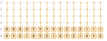
In order to implement the controlled gates, we will turn the Pauli matrices as targets into a multiplexer, and the controlled qubits would be evaluated by a state:
A
c
In[]:=
multiplexer=QuantumCircuitOperator["Multiplexer"@@Keys[pauliDecompose]];
In[]:=
multiplexer["Diagram"]
Out[]=
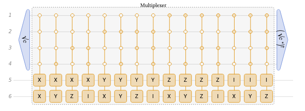
In[]:=
ancillary=QuantumState[Sqrt@Values[pauliDecompose],"Label"->""];
c
In[]:=
QuantumCircuitOperator[ancillary,multiplexer,]["Diagram"]
†
ancillary["Conjugate"]
Out[]=
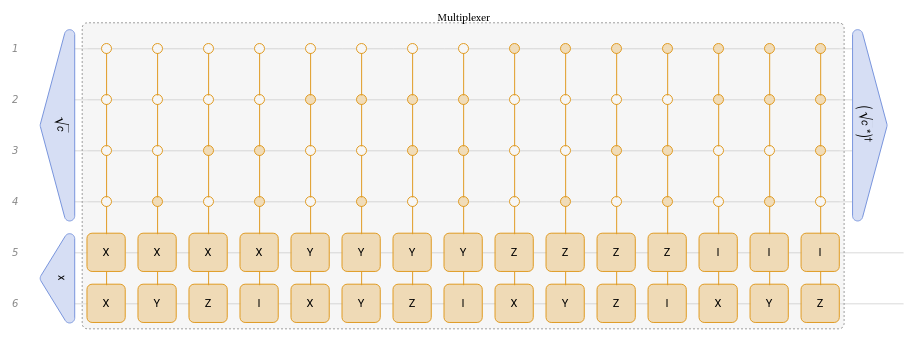
Finally, we would let our vector be evaluated by the multiplexer in our circuit:
x
In[]:=
productCircuit=QuantumCircuitOperator[ancillary,QuantumState[x,"Label"->"x"]->{5,6},multiplexer,];
†
ancillary["Conjugate"]
In[]:=
productCircuit["Diagram",ImageSize->Full]
Out[]=
Evaluate our circuit and check the amplitudes of the resultant state:
In[]:=
productCircuit[]
Out[]=
QuantumState
The result corresponds to the equivalent classical operation:
Quantum Linear Solver Implementation
Quantum Linear Solver Implementation
Now that we learned how to compute the product of a matrix and vector using a quantum circuit, we have a better understanding of how to implement our new variational quantum linear solver.
Initial problem setup
Initial problem setup
As we previously discussed, we need to save the normalization terms, since we will be working with the normalized matrix and vector:
Multiplexer implementation
Multiplexer implementation
Next, implement the multiplexer:
We obtain the first section of the variational circuit for the VQLS:
General symbolic ansatz
General symbolic ansatz
Finally, we implement the circuit and the correspondent state:
Wolfram Quantum Framework quantum states (and measurements) keep the parameters defined in previously used circuits, so it would be optimum to work with the resultant state:
Optimization
Optimization
In other words, this cost function does not ensure that the amplitudes of both states are identical, but rather that they are proportional by a global phase:
Implement the cost functions previously defined, rememer to use the normalized vector b:
Now, let’s optimize the cost function using FindMinimum, with our initial guess as the starting point:
As we can see, FindMinimum is having some difficulty finding the minimal value, so we might switch to NMinimize, which will return a value for the cost function that is very close to zero:
As we can notice, the values are quite close! However, as mentioned earlier, while the probability distributions match, the amplitudes do not necessarily align:
We can verify our result:
Optimization using quantum natural gradient descent
Optimization using quantum natural gradient descent
As explained in a previous example, we can optimize using QuantumNaturalGradientDescent, calculating their correspondent Fubini–Study metric tensor.
The result is quite remarkable: the Quantum Natural Gradient Descent outperforms regular gradient descent and reaches the minimum value in only two steps!
We can verify that the minimization approaches to 0:
As you may have noticed, the probabilities match, but with less precision in this case. However, the amplitudes are completely different, and they even have different signs!
Now, during the process of obtaining the global phase, we observe that the values are not exactly the same. In this case, when we use the mean value of the global phase, we can check that the deviation is small enough for the desired precision.
We can verify our result approximation:
After repeating all the same steps from the previous example, we get a final result that is close to the true result but with slightly less precision. What’s remarkable about this solution is that we achieved it in only two steps! Of course, the results depend heavily on the learning rate eta, so it’s important to fine-tune it to ensure that the optimization is done efficiently.