In[]:=
(*EulerscheKnicklastP2×491https://www.wolfram.com/language/11/differential-eigensystems/index.html.de?footer=lang*)
In[]:=
(*FaxialeDruckkraftaufdenStabEElastizitätsmodulIIFlächenmomentdesStabquerschnittsE*IIBiegesteifigkeitlLängedesStabesxOrty(x)AuslenkungdesStabesausungenickterLageanOrtx0≤x≤l*)Clear[{C1,C2,C3,C4,μ}]y''''+y''==0
F
EII
Out[]=
F
′′
y
II
(4)
y
In[]:=
(*Substitution=(0≤x≤l,μ>0)*)Clear[{C1,C2,C3,C4,μ}]y''''+y''==0
2
μ
F
E*I
2
μ
Out[]=
(4)
y
2
μ
′′
y
In[]:=
(*LösunglautLehrbuchy=C1+C2*x+C3*Sin[μ*x]+C4*Cos[μ*x])zudenRandbedingungenuntenistC1==C2==C4==0nichttrivialeLösungexistiertdannnurwennC3≠0C3*Sin[μ*l]==0Sin[μ*l]==0μn==n==(1,2,3...)führt(unterBeachtungderRandbedingungen)zuderallg.Lösungyn==yn[x]==C3*Sin*x(0≤x≤l)*)Clear[{C1,C2,C3,C4,μ}]DSolve[[x]+[x]0,yy[x],x]
nπ
l
nπ
l
(4)
yy
2
μ
′′
yy
Out[]=
yy(x)-cos(μx)-sin(μx)+x+
c
1
2
μ
c
2
2
μ
c
4
c
3
In[]:=
(*SubstitutionderIntegrationskonstanten*)-cos(μx)-sin(μx)+x+/.{->,->,->,->}
c
1
2
μ
c
2
2
μ
c
4
c
3
c
3
c
1
c
4
c
2
c
2
c
3
c
1
c
4
Out[]=
-cos(μx)-sin(μx)+x+
c
4
2
μ
c
3
2
μ
c
2
c
1
In[]:=
(*LösungunterBeachtungderRandbedingungeny[0]==y[l]==0:keineDurchbiegungandenEndpunkteny''[0]==y''[0]==0:keineBiegemomenteandenEndpunktenTODOliefertnurdietrivialeLösungy[x]===0*)Clear[{C1,C2,C3,C4,μ}]DSolve[[x]+[x]0,yy[0]==0,yy[l]==0,yy''[0]==0,yy''[l]==0,yy[x],x]
(4)
yy
2
μ
′′
yy
Out[]=
{{yy(x)0}}
In[]:=
(*allg.LösungsfunktionderDGLlautLehrbuch*)Clear[{C1,C2,C3,C4,μ}]yy[x_]:=C1+C2*x+C3*Sin[μ*x]+C4*Cos[μ*x](*unterBerücksichtigungderRandbedingungenentstehendiefolgendenvierGleichungen*)
In[]:=
yy[0]==0
Out[]=
C1+C40
In[]:=
yy[l]==0
Out[]=
C1+C2l+C3sin(lμ)+C4cos(lμ)0
In[]:=
yy''[0]==0
Out[]=
-C40
2
μ
In[]:=
yy''[l]==0
Out[]=
-C3sin(lμ)-C4cos(lμ)0
2
μ
2
μ
In[]:=
(*TODOliefertwieDSolvemitRandbedingungenauchnurdietrivialeLösungy[0]==0daauchC3==0geliefertwird*)Clear[{C1,C2,C3,C4,μ}]Solve[C1+C4==0&&C1+C2l+C3Sin[lμ]+C4Cos[lμ]==0-C4==0&&-C3Sin[lμ]-C4Cos[lμ]==0,{C1,C2,C3,C4}]
2
μ
2
μ
2
μ
Out[]=
{{C10,C20,C30,C40}}
In[]:=
(*LösungdereinzigenverbliebenenBestimmungsgleichungfürRandbedingungenlautLehrbuch*)Clear[{C1,C2,C3,C4,μ}]Solve[C3Sin[μl]==0&&C3≠0,μ](*führtimLehrbuchzuμn==(n=1,2,3,...)unddamitzudenEigenlösungenyn==yn[x]==C3*Sinx(0≤x≤l)
nπ
l
nπ
l
Out[]=
μ,μ
In[]:=
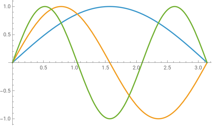
C3=1l=π(*LängegleichT/2*)PlotEvaluateTableC3*Sinx,{n,1,3},{x,0,π},PlotLegends->"Expressions"
nπ
l
Out[]=
1
Out[]=
π
Out[]=