Suppose your world has object types with following probabilities of occurring: 8/10, 2/10, 0
How many object types are in the world? Only counting types that have non-zero probability, our world has 2 object types.
Now suppose the probabilities are 0.8, 0.2, 0.
The count depends on the precision used to do zero-testing on 0.
This counting method produces significantly answers as we vary precision which means it is numerically unstable
How do we count things in a numerically stable way?
This is a real problem when counting dimensions in neural networks because most dimensions are 0 in float32.
When probabilities are all equal, counting is numerically stable. So the non-uniformity that causes problems. Make use of this fact by finding a uniform/isotropic that’s similar in some sense and use it’s dimensionality as the “stable count”.
This is the approach used in Welch-Saitterthwaite approximation to Degrees of Freedom. Suppose linear estimation problem has d independent variables, with per-variable variances,,.., adding up to 1. This problem has similar distribution of residuals as one for an isotropic problem in R dimensions where:
How many object types are in the world? Only counting types that have non-zero probability, our world has 2 object types.
Now suppose the probabilities are 0.8, 0.2, 0.
The count depends on the precision used to do zero-testing on 0.
This counting method produces significantly answers as we vary precision which means it is numerically unstable
How do we count things in a numerically stable way?
This is a real problem when counting dimensions in neural networks because most dimensions are 0 in float32.
When probabilities are all equal, counting is numerically stable. So the non-uniformity that causes problems. Make use of this fact by finding a uniform/isotropic that’s similar in some sense and use it’s dimensionality as the “stable count”.
This is the approach used in Welch-Saitterthwaite approximation to Degrees of Freedom. Suppose linear estimation problem has d independent variables, with per-variable variances
p
1
p
2
p
d
R=R comes up in other places:1. measure of “effective rank” (Bartlett)2. people needed for high chance of shared birthday is approximately 3. number of draws until collision is approximately If R plays the role of d for predicting time until collision on non-isotropic problem, we’d like to1. Evaluate how good this statistic is2. Find a better statistic R1 for predicting mean collision time3. Evaluate R1 in place of d for estimating dimensionality of a learning problemPost below does part 1.TLDR; For many distributions, R is a good proxy of dimensionality, but there’s still room for improvement.Random matrices and GraphData graphs, correspond to distributions with longer time until collision, relative to what we’d expect by using uniform distribution with dimensions d=R.
1
||p
2
||
2Log[2]R
πR/2
How well does R predict time until collision?
How well does R predict time until collision?
In[]:=
Clear["Global`*"];
Initialization
Initialization
multiSpectralPlot[meanTimeToCollision,{uniformSpectra,rminSpectra,rmaxSpectra,powerSpectra,harmonicSpectra},{"uniform","rmin","rmax","power","harmonic"}]
Out[]=
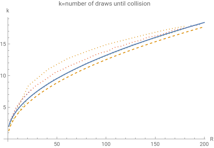


Above are collision times, estimated using answers in this post, evaluated on probability distributions from various distribution families. We can compute exact value using Robert Israel’s formula in this post
Notes:
- formula underestimates the time for finite d
- non-uniform distributions have longer time until collision that uniform with d=R
We can dig deeper into this by plotting residuals for more distribution families
Notes:
-
PiR/2
- non-uniform distributions have longer time until collision that uniform with d=R
We can dig deeper into this by plotting residuals for more distribution families
Distribution families
Distribution families
It’s straightforward to evaluate the formula for a specific kind of distribution, however, the more interesting is to evaluate against a good selection of distributions.
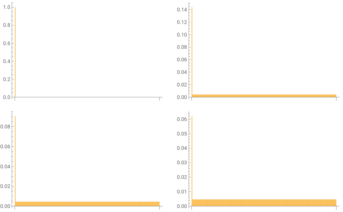
For instance here are “rmin” spectra, these are distribution maximizing for a specific value of R. They try to assign the most mass to one dimension, and split the rest equally.
These extreme distribution was derived by River Li in this post
These appear to have the longest time to collision compared to other distribution with the same R
For instance here are “rmin” spectra, these are distribution maximizing
||p
||
∞
These extreme distribution was derived by River Li in this post
These appear to have the longest time to collision compared to other distribution with the same R
Distributions minimizing/maximizing ||p||∞
Distributions minimizing/maximizing
||p
||
∞
showSpectra[rminSpectra]
Out[]=
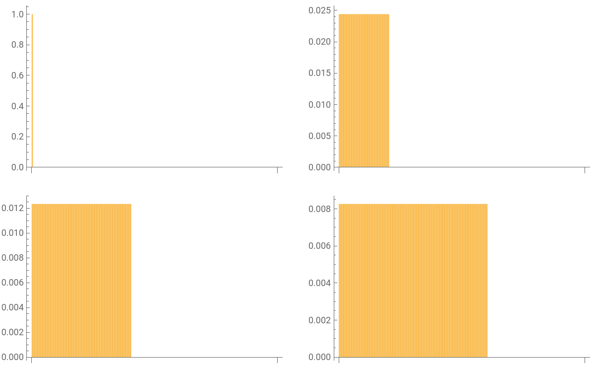
rmax spectra are the opposite of rmin, for fixed R, we try to minimize value of . Such distribution split mass across as many dimensions as possible, and pad the rest with 0s, making it essentially equivalent to uniform
||p
||
∞
showSpectra[rmaxSpectra]
Out[]=
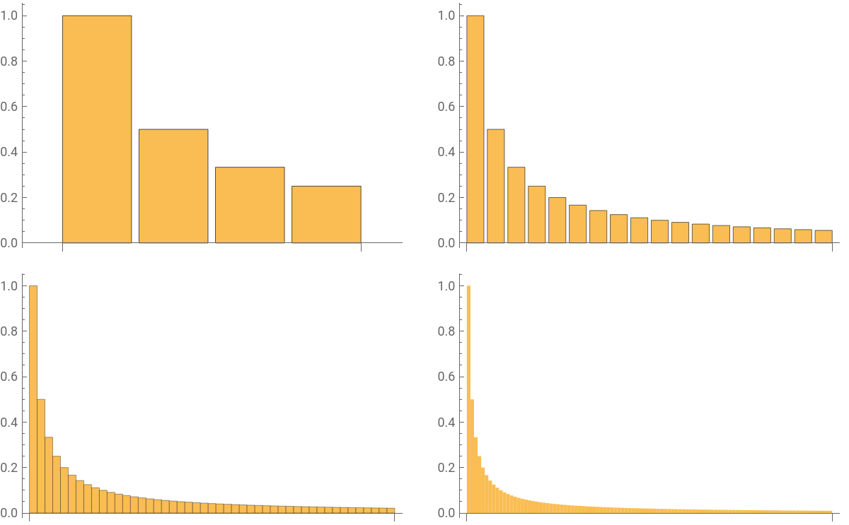
Power spectra are distributions of the form = C for some constant C, p varying and dimensionality fixed
p
i
-p
i
Power-law decaying values
Power-law decaying values
In[]:=
showSpectra[powerSpectra]
Out[]=
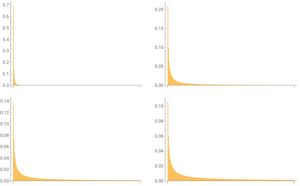
Harmonic spectra are power spectra with p fixed to 1 = C and dimensionality d varying
p
i
-p
i
In[]:=
showSpectra[harmonicSpectra]
Out[]=
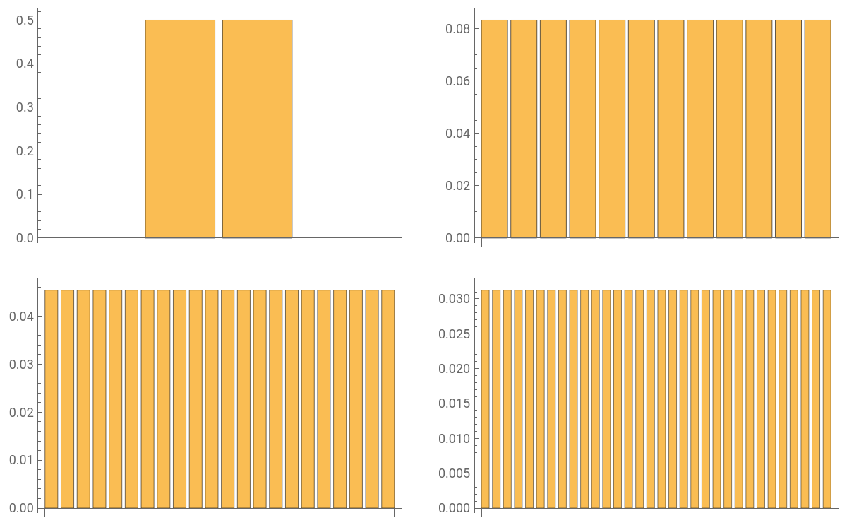
“uniform spectra” are just distribution with all probabilities equal. We use same monte-carlo estimation method for getting their collision time as for other distributions, to get a sense of how far off our estimates are.
In[]:=
showSpectra[uniformSpectra]
Out[]=
Random spectra
Random spectra
Wishart spectra are obtained by looking at eigenvalues of random matrices with Gaussian entries. We get distributions with different values of R by varying the ratio between number of rows and number of columns
product spectra are results of multiplying several Gaussian matrices together with number multiplications varying
Graph spectra
Graph spectra
Graph spectra are spectra are singular values of adjacency matrices of graphs in Mathematica normalized to add up to 1.
Because GraphData these take a while the first time, use “Once[...,Local]” to save it to the local disk
Because GraphData these take a while the first time, use “Once[...,Local]” to save it to the local disk
Residual collision times
Residual collision times
Calculate expected time to collision, subtract expected time to collision for uniform distribution with d=R
We can see that their collision time tends to be longer than what we’d expect by matching this distribution to uniform distribution with same value of R
We can see that their collision time tends to be longer than what we’d expect by matching this distribution to uniform distribution with same value of R
Links
Links
CITE THIS NOTEBOOK
CITE THIS NOTEBOOK
How to count things in numerically stable way
by Yaroslav Bulatov
Wolfram Community, STAFF PICKS, May 9 2023
https://community.wolfram.com/groups/-/m/t/2917025
by Yaroslav Bulatov
Wolfram Community, STAFF PICKS, May 9 2023
https://community.wolfram.com/groups/-/m/t/2917025