ABSTRACT (original article): Since the 19th century, the North Sea sediment system has been subject to a dynamic hydrographic regime and intense human alteration. The Skagerrak serves as the largest depocenter for suspended sediment originating from the North Sea. Thus, deposits in the Skagerrak provide a historical record of potential shifts in the sediment cycle of the North Sea. Despite the availability of mass accumulation rate (MAR) data in the Skagerrak, previous studies focused on steady-state reconstructions and little is known about how these rates may have changed over time. To address this knowledge gap, we present age-depth models based on the natural radionuclide Pb and the anthropogenic time markers Cs, fraction modern C (FC) and mercury (Hg) to determine the MAR before and after the year 1963 at six stations in the deep Skagerrak basin between 434 and 677 m water depth. We applied 1963 as the boundary since this year is constrained by Cs and FC peaks in the sediment cores due to atomic weapons testing and changes in sedimentary Hg contents. Our primary result reveals that the MAR in the deep Skagerrak basin decreased from 0.17 to 0.14 g averaged across the stations. We further simulate the effect of bioturbation on the solid phase profiles by applying a reaction transport model to the data, revealing that the decline in MAR is more pronounced when bioturbation is considered (from 0.17 to 0.09 g ). Decreasing MARs in the Skagerrak basin indicate that the sediment system of the North Sea substantially changed over time. Possible reasons include a shift in the North Sea circulation pattern, enhanced sediment trapping in the Wadden Sea and reduced sediment inputs due to river damming, deepening of harbor channels and coastal protection. However, we stress that our data do not allow for a quantitative analysis of the major driving factors behind the temporal variability of sediment cycling. Hence, we recommend combining our results with information on the provenance of the Skagerrak deposits and integrating the Skagerrak data into larger-scale physical models that consider non-steady state particle transport in the North Sea. CITATION (original article): Spiegel, T., Dale, A. W., Lenz, N., Schmidt, M., Moros, M., Lindhorst, S., Wolschke, H., Müller, D., Butzin, M., Fuhr, M., Kalapurakkal, H. T., Kasten, S., & Wallmann, K. (2025). Mass accumulation rates decreased in the Skagerrak basin over the last 100 years. In Continental Shelf Research (Vol. 286, p. 105411). Elsevier BV. https://doi.org/10.1016/j.csr.2025.105411
210
137
14
14
137
14
-2
cm
-1
yr
-2
cm
-1
yr
Introduction
Introduction
Here, we present the mathematica-based model script related to the publication “Mass accumulation rates decreased in the Skagerrak basin over the last 100 years” (https://doi.org/10.1016/j.csr.2025.105411). The goal was to determine a broad temporal variability of mass accumulation rates (MARs) in the Skagerrak, which is the largest depocenter for sediments in the North Sea. This research goal was set out given the substantial human impacts on the sediment and organic carbon cycle in the North Sea, involving bottom trawling, wind park constructions or coastal protection means. Under “normal” or undisturbed conditions, sediments and the organic carbon can be buried in deeper sediment and effectively escape the short term marine carbon cycle (for millions of years). However, human process may resuspend the material from the seafloor and the once settled organic carbon can be remineralized in the water column. This potentially leads to an enhanced dissolved carbon release into the water column. Higher dissolved carbon concentrations in the water column would mean that less carbon dioxide (CO2) can be taken up from the atmosphere by the North Sea. Hence, the overarching motivation of this project is related to climate change.
The fundamental idea of this specific research was to identify the extent of the sediment resuspension caused by human alterations in the North Sea. Therefore, sediment cores were taken in the Skagerrak basin - the location where a majority of the resuspended material will ultimately deposit. In other words, if there has been any change in the sediment and organic carbon cycle in the North Sea, it should be visible in the depositional record of the Skagerrak. We hypothesized that the MAR in the Skagerrak would increase over time as a result of more sediment resuspension in other areas of the North Sea by human alterations. Hence, identifying the temporal variability of MARs was the main goal of out studies.
The fundamental idea of this specific research was to identify the extent of the sediment resuspension caused by human alterations in the North Sea. Therefore, sediment cores were taken in the Skagerrak basin - the location where a majority of the resuspended material will ultimately deposit. In other words, if there has been any change in the sediment and organic carbon cycle in the North Sea, it should be visible in the depositional record of the Skagerrak. We hypothesized that the MAR in the Skagerrak would increase over time as a result of more sediment resuspension in other areas of the North Sea by human alterations. Hence, identifying the temporal variability of MARs was the main goal of out studies.
Temporal variability of MARs
Temporal variability of MARs
In order to determine the temporal variability of the MARs, we took sediment cores in the Skagerrak and measured the parameters 210Pb, 137Cs, 14C and HG in the sediments at every centimeter from the core top to ca. 40 cm depths. These four parameters are so called “age-depth parameters”. They relate certain depths to certain ages in the sediment core. In simple terms, if one determines that the sediment depths at 5 cm is 10 years old, a sedimentation rate of 0.5 cm/year can easily be calculated. The MAR can then be calculated using the sedimentation rate and by further considering the density of the deposited grains and sediment compaction due to the weight of the overlaying sediments. The MAR is given in the unit grams of sediment/m2/year.
In case of 210Pb, age-depth relationships can be determined because 210Pb naturally decays and we know its decaying behaviour. Half of the 210Pb activity will be decayed, and therefore lost, after 22.3 years (= half life of 210Pb). If we measure a 210Pb activity of 100 dpm/g at the surface (sediment-water column interface) and of 50 dpm/g at 5 cm depth, then we know that 22.3 years have past within the first 5 cm of the sediment, equating to a sedimentation rate of 5cm/22.3years = ca. 0.22 cm/year. In case of 137Cs, 14C and Hg, they are used as a time markers to identify the depth of the year 1963 in the sediment core. In 1963, substantial nuclear weapon testing released 137Cs and 14C into the atmosphere, which can later be tracked as a concentration peak in the sediment cores. Hg was heavily economically utilized since industrialisation with subsequent regulations starting from ca. 1960. Hence, Hg concentrations also show a peak and for simplicity reasons we also refered to it as a 1963 time marker. The 210Pb and the time marker triplet for the year 1963 were used in combination to derive age-depth relationships in the sediment cores.
However, the concentration profiles of the four parameters are not only affected by burial, decay and compaction. Organisms that live, move and build burrows in the sediment can cause mixing of the solid phase profiles complicating their interpretations. In the published manuscript, different methods are presented to still identify a temporal trend of MARs. One of the approaches was to simulate 210Pb, 137Cs, 14C and Hg depth profiles using a reaction transport model simulating the relevant processes. Transport processes in the model included sediment burial, compaction and mixing by organisms (bioturbation), whereas reactions included the decay of the compounds.
The reaction transport model is introduced in the following exemplary for one of the sediment cores “MUC2” in the Skagerrak.
Species considered in the model and measured data
Species considered in the model and measured data
In the following, the species considered in the model and the measured data are listed for the porosity (which is used to simulate sediment compaction) and each of the four age-depth parameters. In the expression {0.5`,0.8688244197050261`}, the first number refers to the sediment depth and the second number to the measured value.
Species considered in the model
Species considered in the model
"Solid species considered in the model conc. in g g dry sediment";sspecies={Age,Pb210ex,Cs137,Hg,C14};
-1
)
Data
Data
"Data for MUC2";"Porosity";"Porosity";Porodata=;"Pb activity in sediment in dpm ";Pb210exdata=;"Cs activity in sediment in dpm ";Cs137data=;"Hg concentration in sediment in ug ";Hgdata=;"F14C fraction modern";C14data=;
210
Excess
-1
g
-1
g
-1
kg
Input parameters
Input parameters
In the following, the general parameter settings of the model are shown. Porosities are later used to determine the effect of compaction. The porosity value represents the amount of water in the pore space between sediment grains in the sediment matrix. Compaction leads to this porewater to be pressed out, reducing the porosity. Hence, the porosity decrease with sediment depth can be used to quantify compaction. Bioturbation refers to sediment mixing of organisms.
Parameter values
Parameter values
"Simulation time in yr,3*L/uf";tmax=200;"Length of the model column in cm";L:=50;"Porosity at sediment-water interface,0.90";P0=0.89;"Porosity after compaction";Pf=0.765;"Parameter for exponential decrease in porosity with depth in 1/cm";px=1/6;"Density of dry solids in g/cm3";ds=2.5;"Bioturbation coefficient at sediment-water interface in cm2/yr";DBio0[t_]:=7;"Bioturbation halfing depth in cm";xBio[t_]:=4.0;"Decay constant of 210Pb in 1/yr";kPb210=0.03114;"Decay constant of 137Cs in 1/yr";kCs137=Log[2]/30.19;"Decay constant of Hg in 1/yr";kHg=0.0000000001;"Decay constant of C14 in 1/yr";kC14=0.0000000001;"Function converting rates from g g dry solids yr into g ( porewater yr";ftcm3[x_]:=ds*(1-Poro[x])/Poro[x]
-1
)
3
cm
-1
)
Change in sedimentation rate (later recalculated to MAR)
Change in sedimentation rate (later recalculated to MAR)
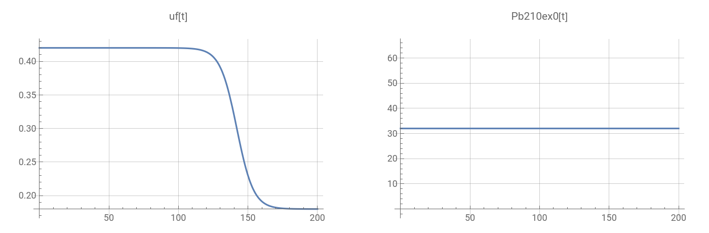
The following equation represents a sigmoid function that changes the sedimentation rate (uf[t_]) from 0.42 before the year 1963 to 0.18 cm/yr after 1963 in this case. This equation is the core of the presented script as it shows the change in sedimentation rates (later recalculated to MARs) at the different stations in the Skagerrak. The parameters Bf1963 and Af1963 were varied until the best possible model fit to the measured data was achieved (here 0.42 and 0.24, respectively). The boundary year 1963 was chosen, since the depth of this year was well-constrained by the time marker triplet in the sediment cores. Hence, the temporal variability in sedimentation rates was determined by virtually splitting the sediment core into two parts, with the artificially set boundary at 1963. This approach does not necessarily reflect natural conditions, as sedimentation rates likely change more gradually probably showing more fluctuations. However, the presented values still accurately represent the average temporal trend in the Skagerrak over the entire timescale (1900 - 2021). For detailed reasons behind the choices and assumptions made, we refer to the published manuscript.
"Burial velocity of solids after compaction in cm/yr";uf[t_]:=Bf1963-Af1963/(1+Exp[((tmax-(2021-1963))-t)/6]);"Burial velocity of solids after compaction in cm/yr";Bf1963=0.42;"Burial velocity of solids after compaction in cm/yr";Af1963=0.24;
Age-depth modeling using 210Pb
Age-depth modeling using 210Pb
The following definition represents a necessary assumption for the method that we applied to model 210Pb, which is referred to as the Constant initial activity (CIC) method. It is one of the most commonly applied methods for age-depth reconstructions with 210Pb. Here, the activity of 210Pb in particles settling at the seafloor (Pb210ex0[t_]) is set to be constant. This value is used to calculate 210Pb fluxes to the seafloor, which is later set as the upper boundary conditions for 210Pb (RR210Pbex). Further methods exist to model 210Pb, i.e. setting a constant 210Pb flux to the seafloor. The details of the different possible approaches and why we chose the CIC method are described in detail in the published manuscript.
"Acitivity of excess 210Pb in particles raining to the seafloor in dpm g dry solids, dpm: disintegrations per minute";Pb210ex0[t_]:=32;
-1
)
The effects of compaction and bioturbation on solid species profiles
The effects of compaction and bioturbation on solid species profiles
The following lines describe the depth and time dependent functions to simulate the effect of compaction on sedimentation rates (us[x_,t_], u0[t_] and MAR[t_]) by using the porosity (Poro[x]) and the effect of bioturbation rates (DBio[x_,t_]) on the solid phase profiles. Please note that the bioturbation rate DBio is expressed as depth and time dependent in the equations below, but no actual time dependency is prescribed for DBio0[t] and xBio[t] - this is an artifact of earlier model runs where the bioturbation rate was set time dependent.
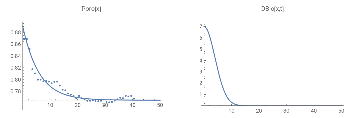
The porosity decline with depth and measured porosity values, the depth variability of bioturbation rates, the sedimentation rate (uf[t]) and the initial 210Pb concentration in settling particles (Pb210ex0[t_]) are plotted below.
The porosity decline with depth and measured porosity values, the depth variability of bioturbation rates, the sedimentation rate (uf[t]) and the initial 210Pb concentration in settling particles (Pb210ex0[t_]) are plotted below.
Depth and time-dependent functions
Depth and time-dependent functions
"Sediment porosity as a function of depth";Poro[x_]:=Pf+(P0-Pf)*Exp[-px*x]"Burial velocity of solids with steady state compaction in cm/yr";us[x_,t_]:=(1-Pf)*uf[t]/(1-Poro[x])"Bioturbation coefficient in sediments in cm2/yr";DBio[x_,t_]:=DBio0[t]*Exp[-x^2/(2*xBio[t]^2)]"Burial velocity of inert solids at sediment-water interface in cm/yr";u0[t_]=uf[t]*(1-Pf)/(1-P0);"Mass accumulation rate of inert particles in g ( seafloor area yr";MAR[t_]=ds*(1-P0)*u0[t];GraphicsGrid[{{Show[Plot[Poro[x],{x,0,L},PlotRangeAll,PlotPoints100,PlotLabel"Poro[x]"],ListPlot[Porodata]],Plot[DBio[x,t],{x,0,L},PlotRange->All,PlotLabel"DBio[x,t]"]}}]
2
cm
-1
)
Out[]=
GraphicsGrid[{{Plot[uf[t],{t,0,tmax},PlotRangeAll,GridLinesAutomatic,PlotLabel"uf[t]"],Plot[Pb210ex0[t],{t,0,tmax},PlotRangeAll,GridLinesAutomatic,PlotLabel"Pb210ex0[t]"]}},ImageSize700]
Out[]=
Timer markers 137Cs, 14C and Hg
Timer markers 137Cs, 14C and Hg
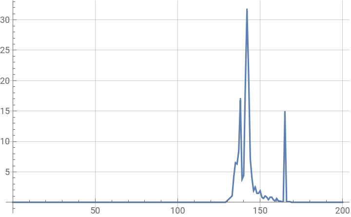
In the following expressions and graphs, the temporally variable concentrations of the three time markers 137Cs, 14C and Hg in particles settling at the seafloor are calculated and shown. To do so, concentration against time data from previously published literature were interpolated. The concentrations in settling particles (Cs0[t_], Hg0[t_] and 14C0[t_]) are later used to calculate the fluxes of the three parameters to the seafloor to set upper boundary conditions.
Time-dependent functions
Time-dependent functions
"Year of sampling";tsamp=2021;"Annual deposition ofCs in the northern hemisphere in Bq (as function of calendar year, Garcia 1998)";dataCs137north=;"Annual deposition ofCs in the northern hemisphere in Bq (as function of model time";Cs137north=;fluxCs137north[t_]:=Interpolation[Cs137north,InterpolationOrder1][t];"Activity of Cs at x = 0 in particles raining to the seafloor in dpm/g";Cs0[t_]:=0.21*fluxCs137north[t];Plot[Cs0[t],{t,0,tmax},PlotRangeAll,GridLinesAutomatic,PlotPoints100]
137
15
10
137
15
10
137
Out[]=
"Annual deposition of Hg in the northern hemisphere in Gg (as function of calendar year)";dataHgnorth=;"Annual deposition of Hg in the northern hemisphere in Gg (as function of model time";Hgnorth=;fluxHgnorth[t_]:=Interpolation[Hgnorth,InterpolationOrder1][t];"Activity of Hg at x = 0 in particles raining to the seafloor in ug/kg";Hg0[t_]:=57*fluxHgnorth[t];Plot[Hg0[t],{t,0,tmax},PlotRangeAll,GridLinesAutomatic,PlotPoints100]
Definition of grid
Definition of grid
Rate terms (decay rates)
Rate terms (decay rates)
In the following, rate terms are defined, i.e. the decay of the different solid phase species. The parameter “Age” is run alongside the other simulations with a one “age” per year increase to check for model consistency.
Depth and time-dependent functions (kinetic rate laws)
Depth and time-dependent functions (kinetic rate laws)
Rate terms for solid phase species
Model simulation based on partial differential equations and boundary conditions
Model simulation based on partial differential equations and boundary conditions
Below, the partial differential equations (PDE) are shown that are used to solve the concentration profiles over depth and time. The equations include the burial, decay, compaction and sediment mixing (bioturbation) of the solid phase species. In order to solve these PDE’s, predefined boundary conditions are necessary. Upper boundary conditions are defined as the fluxes of the different species to the seafloor and lower boundary conditions (at 50 cm sediment depth) as a zero gradient condition. Initial model conditions are then calculated form the boundary conditions. Thereafter, the model solves the PDE’s using the boundary conditions. The resulting model data and measured values for each solid phase species are shown plotted against sediment depth.
Upper boundary condition
Lower boundary conditions at x = L
Initial conditions as calculated from boundary conditions
Solution of PDE
Plots of model results at tmax
CITE THIS NOTEBOOK
CITE THIS NOTEBOOK
Mass accumulation rates decreased in the Skagerrak basin over the last 100 years
by Timo Spiegel
Wolfram Community, STAFF PICKS, February 19, 2025
https://community.wolfram.com/groups/-/m/t/3397403
by Timo Spiegel
Wolfram Community, STAFF PICKS, February 19, 2025
https://community.wolfram.com/groups/-/m/t/3397403