CITE THIS NOTEBOOK: Kinematic analysis and animation of a Stirling cycle engine by David Balandra. Wolfram Community FEB 20 2023.
ORIGINAL ARTICLE: Paul, B., and Krajcinovic, D. (1970). “Computer Analysis of Machines With Planar Motion: Part 1—Kinematics.” ASME. J. Appl. Mech.; 37(3): 697–702. https://doi.org/10.1115/1.3408599.
ORIGINAL ARTICLE: Paul, B., and Krajcinovic, D. (1970). “Computer Analysis of Machines With Planar Motion: Part 1—Kinematics.” ASME. J. Appl. Mech.; 37(3): 697–702. https://doi.org/10.1115/1.3408599.
Kinematics of a Stirling Cycle Engine are solved using NDSolve command, which provides a continuous solution as a function of time for the displacements and velocities of the engine mechanism. The following code can be modified or adapted to analyze similar planar mechanisms
Stirling Engine Schematic Views
Stirling Engine Schematic Views
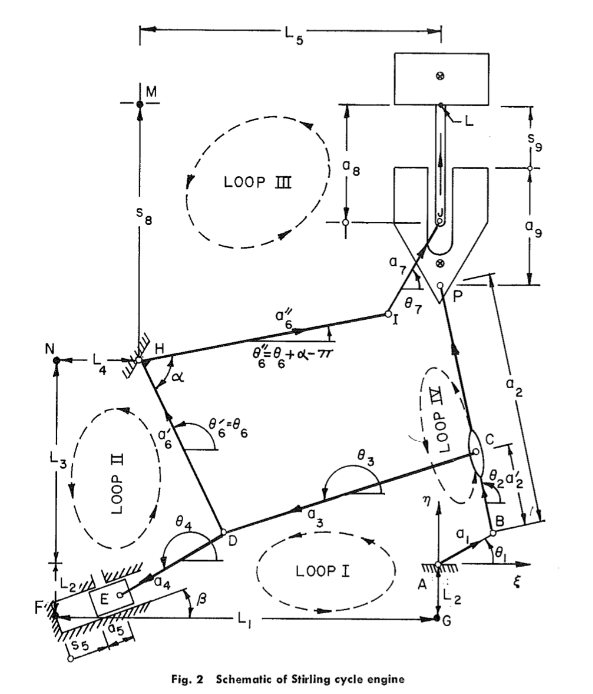
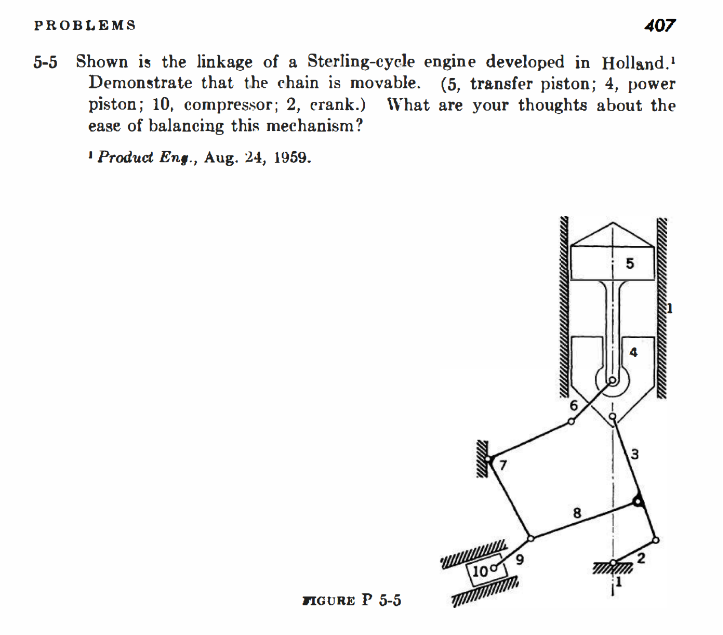
Fig . 2 (left figure) taken from: [1] PAUL, B.; KRAJCINOVIC, D. Computer analysis of machines with planar motion: Part 1—Kinematics. 1970. Link below:
Figure P 5 - 5 (right figure) taken from: [2] HARTENBERG, Richard; DANAVIT, Jacques. Kinematic synthesis of linkages. New York: McGraw-Hill, 1964. Link below:
Displacement Equations
Displacement Equations
In[]:=
Clear[a1,a2p,a3,a4,a5,β,L1,L2,a6p,L4,L3,L2,L5,a6pp,α,a7,a8](*RefertoFig.2abovetoseethefourloops*)l1ξ=a1Cos[θ1[t]]+a2pCos[θ2[t]]+a3Cos[θ3[t]]+a4Cos[θ4[t]]-(a5+L1θ5[t])Cos[β]+L1==0;(*loop1ξ-axis*)l1η=a1Sin[θ1[t]]+a2pSin[θ2[t]]+a3Sin[θ3[t]]+a4Sin[θ4[t]]-(a5+L1θ5[t])Sin[β]+L2==0;(*loop1η-axis*)l2ξ=(L1θ5[t]+a5)Cos[β]-a4Cos[θ4[t]]+a6pCos[θ6[t]]-L4==0;(*loop2ξ-axis*)l2η=(L1θ5[t]+a5)Sin[β]-a4Sin[θ4[t]]+a6pSin[θ6[t]]-(L3+L2)==0;(*loop2η-axis*)l3ξ=a6ppCos[θ6[t]+α-π]+a7Cos[θ7[t]]-L5==0;(*loop3ξ-axis*)l3η=a6ppSin[θ6[t]+α-π]+a7Sin[θ7[t]]+a8-L1θ8[t]==0;(*loop3η-axis*)l4ξ=a1Cos[θ1[t]]+a2Cos[θ2[t]]==0;(*loop4ξ-axis*)l4η=a1Sin[θ1[t]]+a2Sin[θ2[t]]+a9+L1θ9[t]-L1θ8[t]-L3==0;(*loop4η-axis*)
Velocity Equations
Velocity Equations
In[]:=
Dt[{l1ξ,l1η,l2ξ,l2η,l3ξ,l3η,l4ξ,l4η},t,Constants->{a1,a2,a2p,a3,a4,a5,β,L1,L2,a6p,L4,L3,L2,L5,a6pp,α,a7,a8,a9}](*derivingthedisplacementequiationstogetasystemofdifferentialequationstobesolvedwithNDSolvecommand*)
Out[]=
{-a1Sin[θ1[t]][t]-a2pSin[θ2[t]][t]-a3Sin[θ3[t]][t]-a4Sin[θ4[t]][t]-L1Cos[β][t]0,a1Cos[θ1[t]][t]+a2pCos[θ2[t]][t]+a3Cos[θ3[t]][t]+a4Cos[θ4[t]][t]-L1Sin[β][t]0,a4Sin[θ4[t]][t]+L1Cos[β][t]-a6pSin[θ6[t]][t]0,-a4Cos[θ4[t]][t]+L1Sin[β][t]+a6pCos[θ6[t]][t]0,a6ppSin[α+θ6[t]][t]-a7Sin[θ7[t]][t]0,-a6ppCos[α+θ6[t]][t]+a7Cos[θ7[t]][t]-L1[t]0,-a1Sin[θ1[t]][t]-a2Sin[θ2[t]][t]0,a1Cos[θ1[t]][t]+a2Cos[θ2[t]][t]-L1[t]+L1[t]0}
′
θ1
′
θ2
′
θ3
′
θ4
′
θ5
′
θ1
′
θ2
′
θ3
′
θ4
′
θ5
′
θ4
′
θ5
′
θ6
′
θ4
′
θ5
′
θ6
′
θ6
′
θ7
′
θ6
′
θ7
′
θ8
′
θ1
′
θ2
′
θ1
′
θ2
′
θ8
′
θ9
Stirling Engine Parameters
Stirling Engine Parameters
Refer to Fig. 2 in Schematic Views section
In[]:=
a1=2.5;(*in*)a2p=3.5;(*in*)a2=10.5;(*in*)a3=10.5;(*in*)a4=5;(*in*)a6p=8;(*in*)a6pp=10.0;(*in*)a7=6.0;(*in*)L1=17.927;(*in*)L2=3.249;(*in*)L3=8.5;(*in*)L4=5.927;(*in*)L5=12.0;(*in*)α=75Degree;β=20Degree;a5=1;(*in*)a8=5;(*in*)a9=5;(*in*)
Solving for the unknown variables (θ2, θ3, θ4, θ5, θ6, θ7 and θ9)
Solving for the unknown variables (θ2, θ3, θ4, θ5, θ6, θ7 and θ9)
Entry angle θ1 is a known input (θ1 = t) and the input angular velocity is taken as = 1 rad/s. See reference [1].
Equations from Velocity Equations section are rewritten so that they can be solved with NDSolve.
The initial values θ2=π/2, θ3=3.63843, θ4=3.69486, θ5=0.20795, θ6=1.92422, θ7=1.22348, θ8=0.64467, and θ9=0.11474 are taken from reference [1].
′
θ1
Equations from Velocity Equations section are rewritten so that they can be solved with NDSolve.
The initial values θ2=π/2, θ3=3.63843, θ4=3.69486, θ5=0.20795, θ6=1.92422, θ7=1.22348, θ8=0.64467, and θ9=0.11474 are taken from reference [1].
In[]:=
s=NDSolve[{-a1Sin[t]-a2pSin[θ2[t]][t]-a3Sin[θ3[t]][t]-a4Sin[θ4[t]][t]-L1Cos[β][t]0,a1Cos[t]+a2pCos[θ2[t]][t]+a3Cos[θ3[t]][t]+a4Cos[θ4[t]][t]-L1Sin[β][t]0,a4Sin[θ4[t]][t]+L1Cos[β][t]-a6pSin[θ6[t]][t]0,-a4Cos[θ4[t]][t]+L1Sin[β][t]+a6pCos[θ6[t]][t]0,a6ppSin[α+θ6[t]][t]-a7Sin[θ7[t]][t]0,-a6ppCos[α+θ6[t]][t]+a7Cos[θ7[t]][t]-L1[t]0,-a1Sin[t]-a2Sin[θ2[t]][t]0,a1Cos[t]+a2Cos[θ2[t]][t]-L1[t]+L1[t]0,θ2[π/2]==π/2,θ3[π/2]==3.63843,θ4[π/2]==3.69486,θ5[π/2]==0.20795,θ6[π/2]==1.92422,θ7[π/2]==1.22348,θ8[π/2]==0.64467,θ9[π/2]==0.11474},{θ2,θ3,θ4,θ5,θ6,θ7,θ8,θ9},{t,π/2,π/2+2π}](*θ8wasnotrequiredtosolve*)
′
θ2
′
θ3
′
θ4
′
θ5
′
θ2
′
θ3
′
θ4
′
θ5
′
θ4
′
θ5
′
θ6
′
θ4
′
θ5
′
θ6
′
θ6
′
θ7
′
θ6
′
θ7
′
θ8
′
θ2
′
θ2
′
θ8
′
θ9
Out[]=
θ2InterpolatingFunction,θ3InterpolatingFunction,θ4InterpolatingFunction,θ5InterpolatingFunction,θ6InterpolatingFunction,θ7InterpolatingFunction,θ8InterpolatingFunction,θ9InterpolatingFunction


Displacements and velocities plots
Displacements and velocities plots
In[]:=
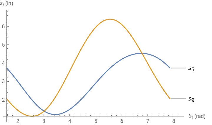
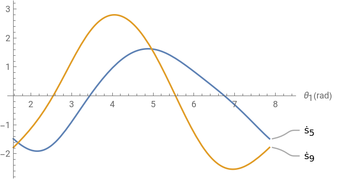
Plot[Evaluate[{L1θ5[t],L1θ9[t]}/.s],{t,π/2,π/2+2π},PlotLabels{"",""},FrameFalse,AxesLabel{"(rad)"," (in)"},PlotRangeAll](*displacementsplots*)Plot[Evaluate[{L1[t],L1[t]}/.s],{t,π/2,π/2+2π},PlotLabels{"",""},FrameFalse,AxesLabel{"(rad)"},PlotRangeAll](*velocitiesplots*)
s
5
s
9
θ
1
s
i
′
θ5
′
θ9
ṡ
5
ṡ
9
θ
1
Out[]=
Out[]=
Compressor parameters for the animation
Compressor parameters for the animation
Assigned parameters for the compressor component: see item 10 in Figure P 5-5 from reference [2]
Stirling Engine Animation
Stirling Engine Animation