There exists a notable interdisciplinary interest in deciphering and characterizing the dynamics and emergent phenomena found within biological media. In this context, lattice models are often utilized to enrich our understanding of these systems [1]. Bearing in mind that these media are generally modeled out of equilibrium and that various diffusive behaviors have been identified [2], this study delves into the exploration of the peculiarities presented by substitution models, and considers how it might be adapted to tackle similar problems.
In the present work, we use the Wolfram Language, cluster size entropy, and mean square displacement to shed light on certain aspects of the dynamics of substitution models. We find that the inherent variability in system size, a fundamental characteristic of substitution systems, impacts our entropy measurements. Even so, cluster size entropy serves as a valuable guide, providing clues about the emerging patterns within the system. Additionally, we find that the system size expands following a pattern of super diffusion.
Although we believe these characteristics may hold relevance for future applications, there remains much to uncover regarding how one might model and understand a biological system using substitution systems.
1. Introduction
1. Introduction
Cellular automata represent dynamic systems wherein space, time, and variables are discretized. In such models, space can be envisioned as a grid of homogeneous cells, each adopting one of a finite number of states — the variables of the system. As the system evolves, these cells change their states following a global rule, which is a function dependent on the cell’s state, the states of its neighboring cells, and time. Cellular automata have proven to be a robust tool for simulating the emergent behavior across a variety of scientific domains, including biology, social science, and physics.
Substitution systems, on the other hand, can be perceived as a variation of cellular automata. Rather than applying a rule to each cell in consideration of its neighbors to advance the system, substitution systems operate on a principle of pattern recognition and replacement. This could involve replacing a single cell or a block of cells. Although substitution systems and cellular automata both encapsulate the principles of local interactions and discrete time steps, the emphasis and mechanisms of evolution exhibit significant differences. Substitution systems are primarily concerned with the substitution of patterns or symbols, whereas cellular automata focus on the state transitions of individual cells, dictated by the states of their adjacent cells.
Despite the diverse applications and successes of cellular automata, one must acknowledge that these simulations are bound by a fixed system size, presenting an inherent limitation. In contrast, substitution systems allow for the exploration of dynamic system size, opening up a new dimension of potential investigations. In this study, we exploit this capability by investigating how system size alters across various substitution systems. Further, inspired by models from the realms of biology and social science, we strive to understand the variability in state group formation within these systems. We utilize two primary tools for our investigation: Cluster Size Entropy () and Mean Square Displacement (MSD).
This notebook is structured as follows: Section 2 outlines the methods and tools utilized in our research. Following this, Section 3 details our results. Lastly, Section 4 provides a summary and synthesis of the findings.
Substitution systems, on the other hand, can be perceived as a variation of cellular automata. Rather than applying a rule to each cell in consideration of its neighbors to advance the system, substitution systems operate on a principle of pattern recognition and replacement. This could involve replacing a single cell or a block of cells. Although substitution systems and cellular automata both encapsulate the principles of local interactions and discrete time steps, the emphasis and mechanisms of evolution exhibit significant differences. Substitution systems are primarily concerned with the substitution of patterns or symbols, whereas cellular automata focus on the state transitions of individual cells, dictated by the states of their adjacent cells.
Despite the diverse applications and successes of cellular automata, one must acknowledge that these simulations are bound by a fixed system size, presenting an inherent limitation. In contrast, substitution systems allow for the exploration of dynamic system size, opening up a new dimension of potential investigations. In this study, we exploit this capability by investigating how system size alters across various substitution systems. Further, inspired by models from the realms of biology and social science, we strive to understand the variability in state group formation within these systems. We utilize two primary tools for our investigation: Cluster Size Entropy (
S
c
This notebook is structured as follows: Section 2 outlines the methods and tools utilized in our research. Following this, Section 3 details our results. Lastly, Section 4 provides a summary and synthesis of the findings.
2. Methodology and Tool Application
2. Methodology and Tool Application
In this study, our focus lies on rules for substitution systems that incorporate the influence of neighboring states within the pattern to be replaced. To conduct this research, we adhere to the following steps:
◼
System Framework: Our study concentrates on one-dimensional systems with periodic boundary conditions.
◼
Neighbor Considerations: We explore rules that consider the influence of immediate neighboring cells. This study includes rules taking into account just one neighbor, as well as rules factoring in two nearest neighbors.
◼
State Diversity: We investigate systems with two and three possible states. When we consider a single neighbor, we study three-state systems to ensure no repetition in neighboring states. Conversely, with two neighbors, we explore four-state systems, keeping in mind the significance of the order of neighboring states.
◼
Evolution Rules and Simulations: For our research, we randomly select 100 evolution rules for each system under study. This selection is executed, and then re-selected randomly 20 times for each system. These simulations use the Wolfram Language and cover ten time steps, providing us with an exploratory overview of a vast number of systems’ behaviors.
◼
Extended Simulations: After obtaining preliminary results from the first phase of simulations, we broaden our analysis by extending the number of time steps for particular cases. This approach allows us to delve deeper into the specific dynamics over a more extended period.
2.1 Neighbor Consideration:
2.1 Neighbor Consideration:
As we mentioned before, for the study of periodic boundary conditions, considering different numbers of interacting neighbors necessitates separate approaches. Specifically, for the single-neighbor case, we employ the function ssRhsNeighbor. This function enables us to model the interaction with a single nearest neighbor within the constraints of periodic boundary conditions.
On the other hand, in the case involving two neighbors, we utilize the function ssFirstNeighbors. This function allows us to take into account both the nearest and second nearest neighbor interactions within the framework of periodic boundary conditions. Both functions, despite their distinct formulations, provide a consistent means of modeling interactions under these boundary conditions.
On the other hand, in the case involving two neighbors, we utilize the function ssFirstNeighbors. This function allows us to take into account both the nearest and second nearest neighbor interactions within the framework of periodic boundary conditions. Both functions, despite their distinct formulations, provide a consistent means of modeling interactions under these boundary conditions.
In[]:=
ssRhsNeighbor[init_List,rules_List]:=Module[{neighborsList,evolutionList},neighborsList=Partition[init,2,1,1];evolutionList=Flatten[neighborsList/.rules]]
In[]:=
ssFirstNeighbors[init_List,rules_List]:=Module[{neighborsList,evolutionList},neighborsList=Partition[init,3,1,2];evolutionList=Flatten[neighborsList/.rules]]
2.2 Cluster Size Entropy (Sc):
2.2 Cluster Size Entropy ():
S
c
A cluster, in discrete terms, is a contiguous group of elements or particles that share a common property, such as a particular state or value. In the context of a cellular automaton, a cluster can be defined as a group of adjacent cells that share the same state. Cluster size entropy () is a statistical measure used to quantify the diversity or variability in the size of clusters within a system [3].
The helps to quantify this complexity by giving us a measure of how evenly the particles in a system are distributed among clusters of different sizes. A high value means that there are many different cluster sizes present in the system, indicative of a complex or disordered state. Conversely, a low value suggests that the particles are predominantly found in clusters of just a few different sizes, indicative of a more ordered state.
This can be particularly relevant for understanding the dynamics of so-called Class 4 cellular automata as per Wolfram’s classification. Class 4 cellular automata exhibit complex, aperiodic behavior and are known to form structures that can interact with each other in intricate ways. This can be seen as a form of aggregation at the mesoscopic scale, and therefore the can provide a useful means of characterizing and quantifying this behavior.
For our subsequent analysis, we define the function ‘clusterSizeEntropy’ under periodic boundary conditions, and it is defined in sections. Notably, the cluster size entropy of an empty set is designated as undefined. This approach will allow us to comprehensively understand the behavior of our system across different conditions and identify any emergent patterns or phenomena.
S
c
The
S
c
S
c
S
c
This can be particularly relevant for understanding the dynamics of so-called Class 4 cellular automata as per Wolfram’s classification. Class 4 cellular automata exhibit complex, aperiodic behavior and are known to form structures that can interact with each other in intricate ways. This can be seen as a form of aggregation at the mesoscopic scale, and therefore the
S
c
For our subsequent analysis, we define the function ‘clusterSizeEntropy’ under periodic boundary conditions, and it is defined in sections. Notably, the cluster size entropy of an empty set is designated as undefined. This approach will allow us to comprehensively understand the behavior of our system across different conditions and identify any emergent patterns or phenomena.
In[]:=
clusterSizeEntropy[{}]=Missing[];clusterSizeEntropy[state_List]:=With[{cluster=Split@state},Entropy@If[cluster[[1]][[1]]!=cluster[[-1]][[1]],cluster,Join[List@Join[cluster[[-1]],cluster[[1]]],Delete[cluster,{{1},{-1}}]]]]
2.3 Diffusion and Anomalous Diffusion:
2.3 Diffusion and Anomalous Diffusion:
Diffusion is a physical process in which particles move and disperse from regions of high concentration to regions of lower concentration. In normal, or Brownian, diffusion, the amount of displacement of a particle over a period of time, as measured by the Mean Squared Displacement (MSD), increases linearly with time. This can be represented by MSD ∝ t, where t is time.
On the other hand, anomalous diffusion is a term used to describe situations where the diffusive behavior deviates from the standard linear pattern. In anomalous diffusion, the MSD may grow faster (super-diffusion) or slower (sub-diffusion) than linear time. This can be represented by the formula MSD ∝ t^α, where α is a constant. If α > 1, it represents super-diffusion, and if α < 1, it represents sub-diffusion.
On the other hand, anomalous diffusion is a term used to describe situations where the diffusive behavior deviates from the standard linear pattern. In anomalous diffusion, the MSD may grow faster (super-diffusion) or slower (sub-diffusion) than linear time. This can be represented by the formula MSD ∝ t^α, where α is a constant. If α > 1, it represents super-diffusion, and if α < 1, it represents sub-diffusion.
2.4 Mean Square Displacement (MSD):
2.4 Mean Square Displacement (MSD):
The Mean Squared Displacement (MSD) is a statistical measure frequently employed in particle physics to quantify the random motion of particles within a media. It is the average of the squares of the displacements of the particles from their initial position over a specified time interval.
In this study, we propose an approach where we equate the initial condition to the initial position, and each rule in a substitution system is analogous to a ‘particle’. This paradigm allows us to investigate how the size of the system—analogous to ‘distance’ in the traditional MSD concept—varies from a given initial condition via the application of different rules. Furthermore, we aim to understand if the initial condition has a significant impact on the evolution of the system size as compared to other initial conditions.
In this study, we propose an approach where we equate the initial condition to the initial position, and each rule in a substitution system is analogous to a ‘particle’. This paradigm allows us to investigate how the size of the system—analogous to ‘distance’ in the traditional MSD concept—varies from a given initial condition via the application of different rules. Furthermore, we aim to understand if the initial condition has a significant impact on the evolution of the system size as compared to other initial conditions.
In[]:=
squareDisplacement[allStates_List]:=With[{initState=Length@allStates[[1]]},Table[(Length@allStates[[i]]-initState)^2,{i,2,Length@allStates}]]
(note that in the squareDisplacement function no mean value was calculated).
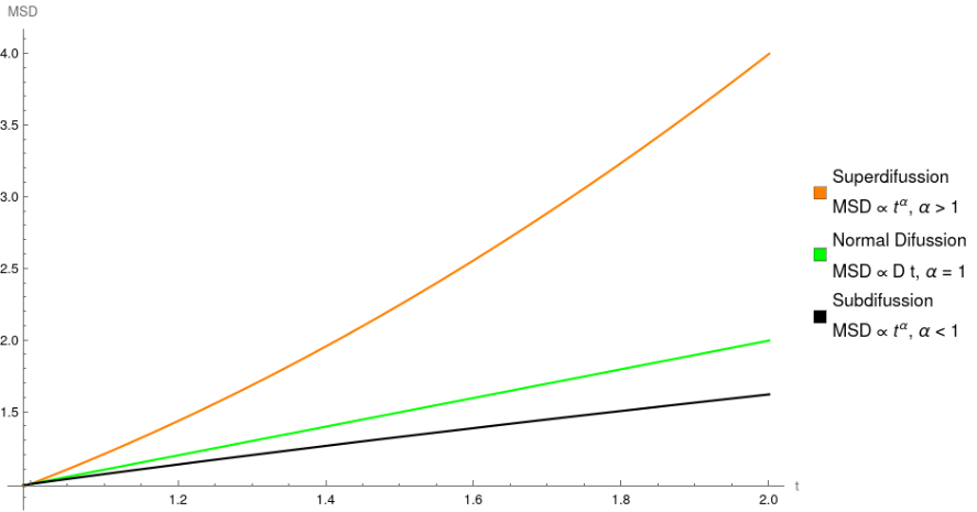
Fig.1: Mean Square Displacement for different types of diffusion.
3. Results
3. Results
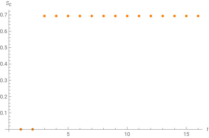
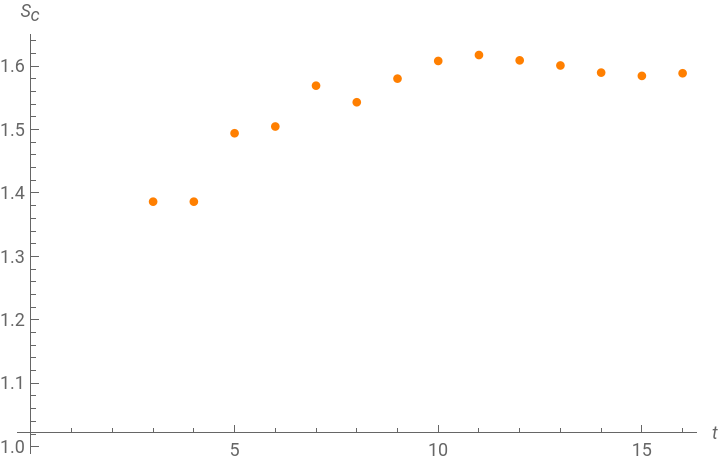
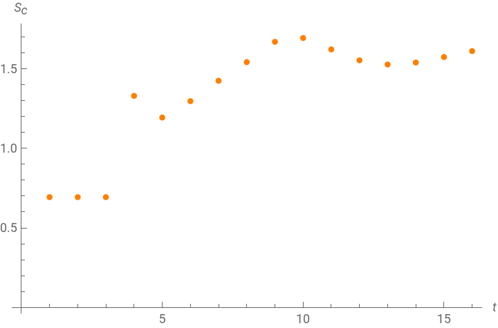
Among the various behaviors observed in our investigation, several noteworthy patterns emerged. Some systems exhibited a constant cluster size entropy value throughout their evolution. Others, however, displayed a transient phase before reaching a steady state. Intriguingly, we also identified systems that oscillate between two or more entropy values in a periodic or asymptotic manner. It is important to note that the steady-state or oscillatory values attained are conditional upon the specific initial states of the system.
Example:
Let’s proceed by considering two possible states, particularly focusing on the scenario where we take into account a single neighboring cell within a specific rule.
Functions to iterate a rule and an initial condition considering one and two neighbors respectively
In[]:=
sSystemOneNeighbor[rule:{(_List->_List)...},init_List,steps_Integer]:=NestList[ssRhsNeighbor[#,rule]&,init,steps]
In[]:=
sSystemFirstNeighbors[rule:{(_List->_List)...},init_List,steps_Integer]:=NestList[ssFirstNeighbors[#,rule]&,init,steps]
Evolution rule, initial conditions, and system simulation
In[]:=
ruleFirstExample={{0,0}{1,1},{0,1}{1},{1,0}{0},{1,1}{1,0}};initialConditionsFirstExample=Tuples[{0,1},3];evaluationsFirstExample=ParallelTable[sSystemOneNeighbor[ruleFirstExample,init,15],{init,initialConditionsFirstExample}];
Plot of Cluster Size Entropy () over time, observing the same rule under varying initial conditions.
S
c
In[]:=
Table[ListPlot[clusterSizeEntropy/@evaluationsFirstExample[[j]],PlotStyle->Orange,AxesLabel->{Style[t],Style[Subscript[S,c]]}],{j,Length@initialConditionsFirstExample}]
Out[]=
,
,
,
,
,
,
,
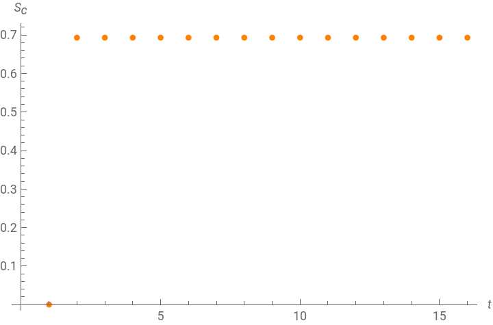
Fig.2: Evolution of cluster size entropy over time under eight different initial conditions in a two-state, one-neighbor system. Each subplot represents one of the eight initial conditions and shows how the cluster size entropy changes over time.
Now, we have selected a particular initial condition and have extended the duration of the evolution process to observe when it reaches equilibrium.
In[]:=
evaluationsFirstExampleExtended=sSystemOneNeighbor[ruleFirstExample,{0,1,0},50];
In[]:=
ListPlot[clusterSizeEntropy/@evaluationsFirstExampleExtended,PlotStyle->Orange,AxesLabel->{Style[t,20],Style[Subscript[S,c],20]},LabelStyle->{FontSize->15},ImageSize->Large]
Out[]=
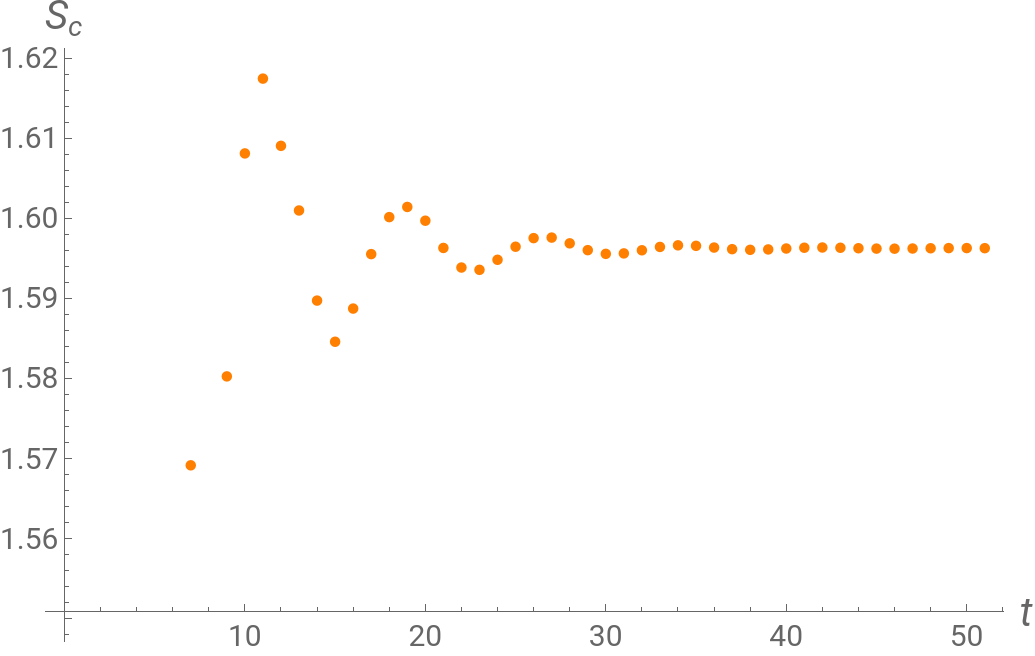
Fig.3: Evolution of cluster size entropy over time considering the initial condition {0, 1, 0} and the rule {0,0}{1,1},{0,1}{1},{1,0}{0},{1,1}{1,0}.
Evolutionary pattern present in the system.
In[]:=
ArrayPlot[evaluationsFirstExampleExtended[[;;11]],ColorRules->{0->Green,1->Orange},Mesh->Automatic,ImageSize->Full]
Out[]=

Fig.4: Evolution pattern of the substitution system considering the initial condition {0, 1, 0} and the rule {0,0}{1,1},{0,1}{1},{1,0}{0},{1,1}{1,0}.
But what does it mean for the cluster size entropy to reach a constant value? In simple terms, it indicates that the number of clusters in the system remains constant - no further structures appear or disappear within the system, regardless of whether their size continues to increase or decrease. This becomes more apparent in the following example.
Let’s consider the evolution rule:
Under the initial condition:
Considering 50 steps of evolution
Fig.5: Evolution of cluster size entropy over time considering the initial condition {0, 1, 0} and the rule {0,0}{0},{0,1}{0,0},{1,0}{1,1},{1,1}{1}.
Evolution pattern; second example:
Fig.6: Evolution pattern of the substitution system considering the initial condition {0, 1, 0} and the rule {0,0}{0},{0,1}{0,0},{1,0}{1,1},{1,1}{1}.
As anticipated, when considering more states, the entropy tends to be higher, and new behaviors emerge in the cluster size entropy. In the following examples, we consider three states and a single neighbor. We identify patterns of oscillation among three entropy values, followed by oscillation between two values, and subsequently another oscillation between two values that appears to asymptotically converge.
Fig.7: Evolution of cluster size entropy over time considering the initial condition {1, 1, 1} and the rule {0,0}{0},{0,1}{0,2},{0,2}{1,1},{1,0}{1},{1,1}{2,1},{1,2}{1,0},{2,0}{2,0},{2,1}{},{2,2}{1,2}.
Evolution pattern; third example:
Fig.8: Evolution pattern of the substitution system considering the initial condition {1, 1, 1} and the rule {0,0}{0},{0,1}{0,2},{0,2}{1,1},{1,0}{1},{1,1}{2,1},{1,2}{1,0},{2,0}{2,0},{2,1}{},{2,2}{1,2}.
Rules, initial condition, and evolution for our fourth example
Fig.9: Evolution of cluster size entropy over time considering the initial condition {0, 1, 0} and the rule {0,0}{1},{0,1}{2,1},{0,2}{0,2},{1,0}{1,2},{1,1}{2,0},{1,2}{2},{2,0}{},{2,1}{0,1},{2,2}{0}.
Evolution pattern; fourth example:
Fig.10: Evolution pattern of the substitution system considering the initial condition {0, 1, 0} and the rule {0,0}{1}, {0,1}{2,1}, {0,2}{0,2}, {1,0}{1,2}, {1,1}{2,0}, {1,2}{2}, {2,0}{}, {2,1}{0,1}, {2,2}{0}.
Rules, initial condition, and evolution for our fifth example
Fig.11: Evolution of cluster size entropy over time considering the initial condition {0, 2, 1} and the rule {0,0}{2,1}, {0,1}{1}, {0,2}{0,0}, {1,0}{1,0}, {1,1}{}, {1,2}{1,1}, {2,0}{2}, {2,1}{1,2}, {2,2}{0,1}.
Evolution pattern; fifth example:
Fig.12: Evolution pattern of the substitution system considering the initial condition {0, 2, 1} and the rule {0,0}{2,1}, {0,1}{1}, {0,2}{0,0}, {1,0}{1,0}, {1,1}{}, {1,2}{1,1}, {2,0}{2}, {2,1}{1,2}, {2,2}{0,1}.
In all the variations of the system that we have studied, the mean square displacement (MSD) shows the same behavior. We have observed that the MSD of the system size evolves in a manner similar to anomalous diffusion. By fitting the curve corresponding to anomalous diffusion, x^α, we observe that the value of α depends on the initial condition. However, it is always greater than one, which is consistent with super-diffusion.
Definition of substitution system parameters: setting the number of rules, identifying all possible substitutions, neighbors, and establishing initial conditions.
Random generation of rules
System evolution
Calculation of square displacement
Calculation of Mean square displacement
Plot of Mean Square Displacement (MSD) over time considering three states.
Fig.13: Evolution of the Mean Square Displacement (MSD) over time under twenty-seven different initial conditions in a system considering three states and one neighbor. Each subplot represents one of the twenty-seven initial conditions and illustrates how the MSD follows a non-linear behavior with respect to time in a very short diffusive regime. Notably, these plots suggest that the non-linear pattern is characteristic of super-diffusive behavior (see Fig.[1]).
Alpha coefficient estimation from data fitting.
4. Summary
4. Summary
Throughout the course of this research, we have demonstrated how substitution systems can be characterized by employing the cluster size entropy and the mean square displacement. We discovered that while the cluster size entropy can serve as an effective tool to garner a qualitative picture of the system’s behavior, it is paramount to consider how changes in the system’s size can influence its measure. Moreover, during the course of this study, we observed a pattern of system size growth that mirrors super-diffusion.
It is important to note that our exploration of diffusion was confined to a very short time diffusive regime, a factor that should be taken into account when considering the implications of our findings and their potential future applications. The impact of this limitation on our results and potential mitigation strategies needs to be explored in future research.
We also acknowledged that the number of rules explored in this study is quite small, which suggests the need for a comprehensive investigation to further delve into this aspect. Even though it’s true that substitution models can generate patterns of varying complexity, it’s important to note that for future applications, we need a sophisticated interpretation of metrics such as the mean square displacement. In addition, we need to identify a rule that can simulate some natural phenomenon, and define parameters that allow us to test diverse hypotheses or perform different measurements on our system.
Despite the challenges being numerous, they do not appear insurmountable, as similar difficulties have been previously overcome in cellular automata systems. With a more exhaustive exploration of rules and a refined understanding of system measurements, we look forward to discovering what more these substitution systems have to reveal.
Keywords
Keywords
◼
Substitution Systems
◼
Neighbor-dependent
◼
Cluster Size Entropy
◼
Mean Square Displacement
Acknowledgment
Acknowledgment
The author acknowledges Stephen Wolfram for proposing the study of neighbor-dependent substitution systems and expresses gratitude to Eric James Parfitt for assisting with the code, corrections, and overall support in preparing this document. Special thanks are extended to Yennifer Betancourt Zúñiga for her emotional support and love throughout the project. Felipe Barros Cárdenas is also thanked for providing valuable comments and insights. Additionally, the author expresses gratitude to the Department of Physics and the Postgraduate Directorate at the University of Concepción for their financial support, which enabled their participation in this school.
References
References
◼
[1] Soto, Rodrigo and Golestanian, Ramin. Run-and-tumble dynamics in a crowded environment: Persistent exclusion process for swimmers. Phys. Rev. E 89, 012706. http://dx.doi.org/10.1103/PhysRevE.89.012706
◼
[2] Reverey, J., Jeon, JH., Bao, H. et al. Superdiffusion dominates intracellular particle motion in the supercrowded cytoplasm of pathogenic Acanthamoeba castellanii. Sci Rep 5, 11690 (2015). https://doi.org/10.1038/srep11690
◼
[3] Gandica, Y. and Charmell, A. and Villegas-Febres, J. and Bonalde, I. Cluster-size entropy in the Axelrod model of social influence: Small-world networks and mass media. Phys. Rev. E 84, 046109 (2011). http://dx.doi.org/10.1103/PhysRevE.84.046109
◼
[4] Wolfram, S. (2002). A New Kind of Science. Wolfram Media. pp. 85-86. www.wolframscience.com
CITE THIS NOTEBOOK
CITE THIS NOTEBOOK
Exploring neighbor dependent substitution systems using cluster size entropy and MSD
by Jim Tortella
Wolfram Community, STAFF PICKS, July 12, 2023
https://community.wolfram.com/groups/-/m/t/2959211
by Jim Tortella
Wolfram Community, STAFF PICKS, July 12, 2023
https://community.wolfram.com/groups/-/m/t/2959211