Introduction
What are Raven’s Progressive Matrices (RPMs)?
What are Raven’s Progressive Matrices (RPMs)?
Raven’s Progressive Matrices are a nonverbal test typically used to measure general human intelligence and abstract reasoning and is regarded as a non-verbal estimate of fluid intelligence. It is one of the most common tests administered to both groups and individuals ranging from 5-year-olds to the elderly. It typically comprises 60 multiple choice questions, listed in order of increasing difficulty. This format is designed to measure the test taker’s reasoning ability.
The matrices are composed of a number of elements, which are altered in a fixed pattern to generate a series of matrices. For normal RPM testing, a set of possible solutions is provided and the test taker then attempts to select the correct answer from the possible solution set. In the current form of this application, the computer attempts to determine what the next matrix in the pattern will be without a solution set from which to sample, meaning that the computer is selecting from all possible solutions. This makes the solution more difficult to determine. In the final project, a set of possible solutions will be generated from which the computer will select the most likely answer.
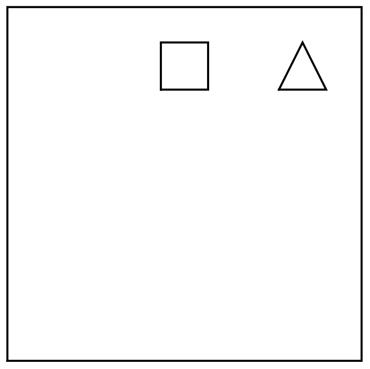
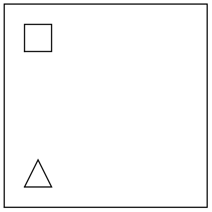
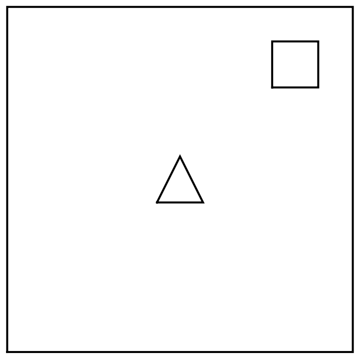
The currently implemented attributes for movement of shapes within the matrices are Movement and Bounce. Movement moves a fixed number of steps (currently an integer in the range of -1 to 1) in the horizontal and/or vertical direction, wrapping to the same row/column when it passes an edge. Bounce similarly moves a fixed number of steps (currently an integer in the range of -1 to 1) in the horizontal and/or vertical direction, however when it reaches an edge the direction of movement is reversed.
Code
Code
Sample RPMs
Sample RPMs
Graphical Representation
Graphical Representation
Below is a sample RPM sequence, showing the eight matrices followed by the solution. The position of each element is stored in the RPM, with the positions assigned 1 through () where the bottom left corner is 1, and the top right corner is
2
size
().
2
size
In[]:=
tmp=createRPMArray[3];{drawRPMArray[tmp,3],drawRPMSolution[tmp,3]}
Out[]=
,
,
,
,
,
,
,
,
Symbolic Representation
Symbolic Representation
In order to minimize memory usage and increase classification speed, the RPMs are converted to a 3x3 bitmap representation, with colours representing the shapes, and the positions reflected as above.
In[]:=
{imagesFromRPM[tmp,3]->solutionImageForRPM[tmp,3]}
Out[]=
,

,

,

,
,
,
,
This is done for each position of the matrix, yielding a symbolic representation of the matrices .
Below is the internal representation of the array:
This is done for each position of the matrix, yielding a symbolic representation of the matrices .
Below is the internal representation of the array:
In[]:=
tmp
Out[]=
{{{Position8,Movement{-1,0},Position7,Movement{-1,0},Position9,Movement{-1,0},Position8,Movement{-1,0},Position7,Movement{-1,0},Position9,Movement{-1,0},Position8,Movement{-1,0},Position7,Movement{-1,0}},Position9,Movement{-1,0}},{{Position9,Movement{1,1},Position1,Movement{1,1},Position5,Movement{1,1},Position9,Movement{1,1},Position1,Movement{1,1},Position5,Movement{1,1},Position9,Movement{1,1},Position1,Movement{1,1}},Position5,Movement{1,1}}}
Classification
Classification
Training Example
Training Example
The classifier is trained using the LogisticRegression method. In order to generate a training set, a number of RPM’s can be generated. For a simple example, we can generate 100 RPM’s with the following:
In[]:=
trainingSet=Table[createRPMArray[3],100];
Having generated a table of 100 RPM’s, we can then create a set of rules out of these RPM’s as follows:
In[]:=
trainingAssociation=<||>;AssociateTo[trainingAssociation,imagesFromRPM[trainingSet[[#]],3]->solutionImageForRPM[trainingSet[[#]],3]]&/@Range[Length[trainingSet]];
You can see the first three rules in this association below.
In[]:=
trainingAssociation[[;;3]]
Out[]=
,

,

,

,
,
,
,
,
,

,

,

,
,
,
,
,
,

,

,
,

,
,
,
The association is then converted to a list of rules for use with Classify using the Normal function.
In[]:=
normalTrainingAssociation=Normal[trainingAssociation];
This set of rules is then passed to the classify function with the options MissingValues -> None and Method -> “LogisticRegression”:
In[]:=
demoClassifier=Classify[normalTrainingAssociation,MissingValueSynthesis->None,Method->"LogisticRegression"]
Out[]=
ClassifierFunction


Which yields a classifier for this training set.
Training Set
Training Set
The accuracy of the classifier is dependent upon the size of the training set. There are 81 possible outputs (2 symbols with 9 positions each), however there are a great many more possible ways to reach those solutions. With a 3x3 matrix, there are 8,649 possible sequences. Training on the full set amounts to simply memorizing the sequences and their outcomes, therefore the training size was adapted in order to find a minimum training size with a high probability of correct answers.
The full set of sequences is generated randomly in order to ensure a random order to the example set. The first n items of the set are then selected as training examples, where n is the first parameter passed to the testWithSamples function. The second parameter is the size of the matrix, which is always square. The classifier is trained with the training examples, and a table is generated which tests 1000 random examples that are not a part of the training data. This entire process, including generation of the examples, is repeated ten times. testWithSamples then returns a table with 10 numbers, each expressing the percentage of successfully classified examples of the 1000 random examples tested.
The full set of sequences is generated randomly in order to ensure a random order to the example set. The first n items of the set are then selected as training examples, where n is the first parameter passed to the testWithSamples function. The second parameter is the size of the matrix, which is always square. The classifier is trained with the training examples, and a table is generated which tests 1000 random examples that are not a part of the training data. This entire process, including generation of the examples, is repeated ten times. testWithSamples then returns a table with 10 numbers, each expressing the percentage of successfully classified examples of the 1000 random examples tested.
Example
Example
In[]:=
result=testWithSamples[2500,3]
Out[]=
{1.,1.,1.,1.,1.,1.,1.,1.,1.,1.}
As can be seen in the output above, with 2500 training examples, a LogisticRegression classifier is able to achieve 100% accuracy for this set.
Below, a result done with 1000 training examples provides significantly lower accuracy.
Below, a result done with 1000 training examples provides significantly lower accuracy.
In[]:=
result2=testWithSamples[1000,3]
Out[]=
{1.,0.6,0.9,0.8,0.9,0.8,1.,0.7,0.8,0.9}
Next Steps
Next Steps
Increased Domain
Increased Domain
The RPMs being generated thus far are fairly simple, with only two types of movement. More objects are to be added, as well as support for rotation and filled/unfilled objects.
Addition of “Red Herring” objects
Addition of “Red Herring” objects
In more complex RPMs used in the real world, objects are sometimes added which move randomly and do not follow a fixed pattern. The ideal system would be able to identify and disregard these objects. This amounts to noise in the training set, which I anticipate will reduce accuracy. I intend to see how much noise can be added before the accuracy of the classifier becomes too low to be useful.