Abstract: This project investigates the solutions to the PDE: u(t,x)u(t,x)-a(u(t,x)+b)(u(t,x)-b)u(t,x). Because of a non-stable equilibrium at , the system shows chaotic behavior. Interesting structures are observed in numerically computed solutions, and their features are analyzed for different a and b parameters. Time-independent version of the above equation is studied and solutions are used as initial conditions - resulting in non-stable equilibrium states.
2
∂
t
2
∂
x
u0
u(t,x)
Introduction
Introduction
Inspiration
Inspiration
One of the most basic important PDE equations is the wave equation:
2
∂
t
2
c
2
∂
x
This could describe a wave traveling in a nonelastic medium.
To introduce an elastic medium, one should solve:
To introduce an elastic medium, one should solve:
2
∂
t
2
c
2
∂
x
In a more general case, one can explore the solutions of equations of the form:
2
∂
t
2
c
2
∂
x
Narrowing down the search
Narrowing down the search
The vast space of possible f functions provides a plethora of possible solutions.
Even constraining it to a 3rd degree polynomial, leaves plenty of systems to explore, each behaving it’s own complicated manner.
For simplicity, the c constant will be set to 1 and the numerical solutions will be calculated over a fixed region of, mostly with Dirichlet boundary conditions.
Furthermore, for reasons explained in the next chapter, this project will focus on functions in the form of:
Even constraining it to a 3rd degree polynomial, leaves plenty of systems to explore, each behaving it’s own complicated manner.
For simplicity, the c constant will be set to 1 and the numerical solutions will be calculated over a fixed region of
-5≤x≤5
Furthermore, for reasons explained in the next chapter, this project will focus on functions in the form of:
f(u)au(u-b)(u+b)
Physical wave equations
Physical wave equations
Linear wave equations
Linear wave equations
When introduced to the concept of wave equations, ropes and strings are used as props by teachers. This analogy will be useful for getting familiar with the plots generated in this project.
Let’s start by defining a function to generate appropriate initial conditions for solving the basic wave equation numerically.
The function returns a traveling wave for each triplet in the input:
u0multipleV
{position,velocity,amplitude}
In[]:=
u0multipleV[impactXs_,a_:4]:={Function[x,Total[Map[(#[[3]]*E^(-a(x-#[[1]])^2))&,impactXs]]],Function[x,Total[Map[2*a*#[[2]]*#[[3]]*E^(-a)(x-#[[1]])&,impactXs]]]}
2
(#[[1]]-x)
Specify the size and length of the simulation:
In[]:=
x0=5;ropetmax=10;
Specify the boundary conditions:
In[]:=
bc={u[t,-x0]==0,u[t,x0]==0};
Give the initial conditions:
In[]:=
{u0R,du0dtR}=u0multipleV[{{-1,1,1}}];
Use to solve the PDE:
In[]:=
ropeSol=NDSolveValue[Flatten@{D[u[t,x],t,t]==D[u[t,x],x,x],u[0,x]==u0R[x],D[u[t,x],t]==du0dtR[x]/.t0,bc},u,{t,0,ropetmax},{x,-x0,x0},Method{"MethodOfLines","SpatialDiscretization"{"TensorProductGrid","DifferenceOrder""Pseudospectral","MinStepSize"->0.005,"MaxStepSize"->0.6}}]
Out[]=
InterpolatingFunction


For solving this project’s PDEs method of lines is used. Information about the method is available on this Documentation page. The important part of specifying the Method are the MinStepSize and MaxStepSize values, which control how detailed and computationally expensive the simulation will be.
The solution is an interpolating function u, which takes two arguments: t and x. While thinking of the solution as the evolution of a 1D string in time is more intuitive, plotting it as a 2D density plot allows for more effective display of results.
Below are two ways to visualize the solution:
Define two plotting functions:
In[]:=
myColorFunction=Function[x,Blend[{{-5,Magenta},{-2,Purple},{-1,Blue},{0,Black},{1,Red},{2,Orange},{3,Yellow},{4,White}},x]];
In[]:=
plotWavePDEsolution[ufun_,x0_,tmax_,tmin_:0]:=DensityPlot[ufun[t,x],{x,-x0,x0},{t,tmin,tmax},PlotRangeAll,PlotLegends->Automatic,FrameLabel->{"x","t"},ColorFunction->myColorFunction,ColorFunctionScaling->False,MaxRecursion->5,PerformanceGoal->"Quality"]
In[]:=
ropePlot=Evaluate@plotWavePDEsolution[ropeSol,x0,ropetmax];Manipulate[Row[{Plot[ropeSol[t,x],{x,-x0,x0},PlotRange->{-4,4},AxesLabel->{"x","u"},ImageSize->300,MaxRecursion->3,PlotPoints->10],Show[ropePlot,Epilog->{LightGreen,Line[{{-x0,t},{x0,t}}]},ImageSize->300]}],{t,0,ropetmax},SaveDefinitions->True]
Out[]=


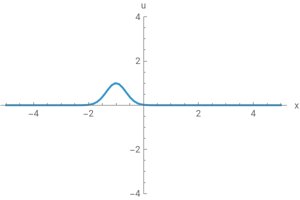
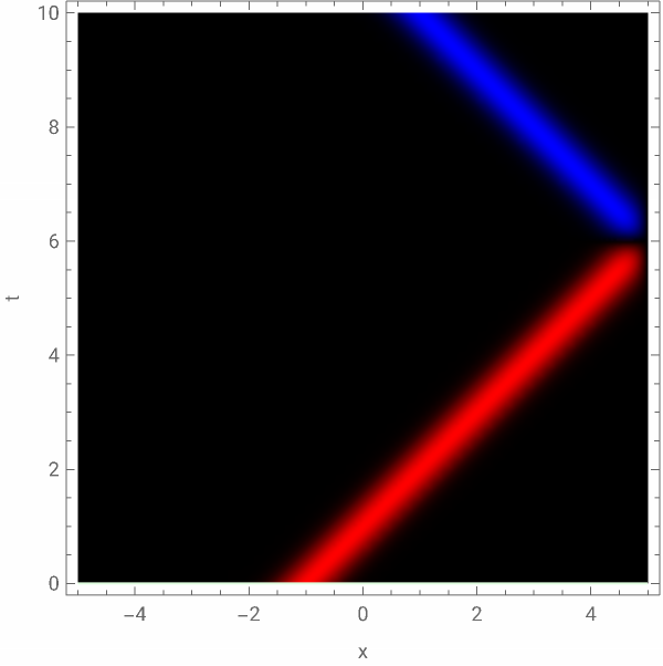

This behavior is what we expect of a basic wave equation with Dirichlet boundary conditions. The plot on the right is represents the entire solution with color representing the displacement u, the green line indicates what slice of that plot was used to create a frame of the animation on the left side.
Now let’s look at how the solution changes, when we introduce linear elasticity by changing the equation to:
2
∂
t
2
∂
x
In[]:=
stringtmax=20;stringSol=NDSolveValue[Flatten@{D[u[t,x],t,t]==D[u[t,x],x,x]-5u[t,x],u[0,x]==u0R[x],D[u[t,x],t]==du0dtR[x]/.t0,bc},u,{t,0,stringtmax},{x,-x0,x0},Method{"MethodOfLines","SpatialDiscretization"{"TensorProductGrid","DifferenceOrder""Pseudospectral","MinStepSize"->0.005,"MaxStepSize"->0.6}}]
Out[]=
InterpolatingFunction
In[]:=
stringPlot=Evaluate@plotWavePDEsolution[stringSol,x0,stringtmax];Manipulate[Row[{Plot[stringSol[t,x],{x,-x0,x0},PlotRange->{-4,4},AxesLabel->{"x","u"},ImageSize->300,MaxRecursion->3,PlotPoints->10],Show[stringPlot,Epilog->{LightGreen,Line[{{-x0,t},{x0,t}}]},ImageSize->300]}],{{t,10},0,stringtmax},SaveDefinitions->True]
Out[]=
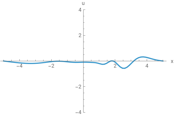
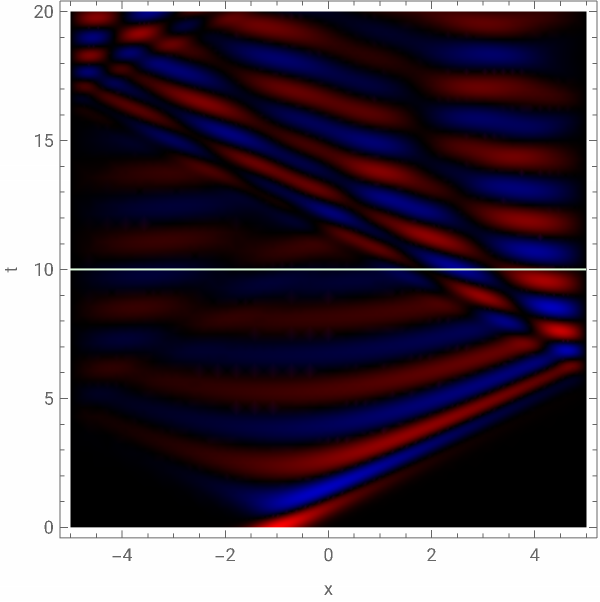

Naturally, the system behaves differently - a small distrurbance propagates to the entire string and causes oscillations, as it happens in a guitar string.
Force from displacement is linear in a harmonic oscillator, and the harmonic potential is a quadratic function:
Force from displacement is linear in a harmonic oscillator, and the harmonic potential is a quadratic function:
Beyond linearity
Beyond linearity
But for different materials, systems or large displacements, exceptions from Hooke’s law appear in Physics. For example, one could imagine a material where elasticity is described with a 5th degree polynomial:
As can be seen above, while the Force from Displacement plot looks rather interesting, the potential looks similar to the harmonic case - and thus the system shows similar behavior. There is a major difference in the exact numerical values, especially for multiple traveling waves (because superposition does not hold), but the overall results are the same - oscillations.
This is as much complexity as one can get from a system representing an elastic medium. While non-monotonous Force(Displacement) functions can to some degree be observed in nature, it is hard to have an intuition for a system with multiple potential minima - as then for some displacements the force would have to be attractive, not repulsive. This is why, while building on physical intuition, the project will explore systems constructed purely in search for complex behavior.
For choosing a system to explore in this project the following assumptions were made:
Stability
Stability
The potential should tend to infinity for large displacements, to ensure the function doesn’t blow up. In the case of polynomials, this means the leading term in the PDE should be u to an odd power, with a negative sign.
Symmetry
Symmetry
While arbitrary, this project seeks to explore systems with symmetry about zero. This means antisymmetric f functions, which corresponds to polynomials with odd terms only. An argument can be made that non-symmetric systems can show even more interesting behavior, however in Physics it is natural to expect symmetries and common to use them as base for interpretation of results.
Simplicity
Simplicity
An infinite number of polynomials can be investigated. Furthermore any function of u can be added and potentially produce complex patterns. But following the idea behind cellular automata, the most exciting complexity comes from the simplest of rules. This is why the project investigates the simplest non-trivial polynomial that satisfies above conditions: a third degree polynomial.
Symmetric nonlinear wave equation
Symmetric nonlinear wave equation
A new kind of wave equation
A new kind of wave equation
Because of reasons explained above, the project investigates the equation in form of:
Where the polynomial expands to:
Let’s visualize the polynomial and the resulting potential:
Example solutions
Example solutions
Let’s introduce tools to compute and visualize solutions:
To generate initial conditions that induce symmetry breaking, let’s define a function generating an interpolating function based on some noise:
(satisfies Dirichlet boundary conditions)
(satisfies Dirichlet boundary conditions)
Visualize the result:
Generate a polynomial from u:
General solver function, that can take any f function, and has option for Dirichlet/Periodic BC:
(for more specific cases it can be beneficial to use ParametricNDSolve)
(for more specific cases it can be beneficial to use ParametricNDSolve)
Let’s prepare some initial conditions:
Calculate and plot solutions:
For relatively low a and b (both equal 1) the resulting plot is not very exciting. Some oscillations can be seen and the solution tends to stay in the positives, with some exceptions near the boundaries. But let’s check how the systems behavior changes with increased a and b parameters.
As can be seen on these plots, drastically increasing a increases the frequency of oscillations, but more importantly, causes the sign of u to change over time, which on a 2D density plot results in domain-like structures. There’s few of them at any given t but it’s worth noting how u can become positive, after being negative for any x (as it does around t = 20 and t = 25).
Now let’s look what changes when the b parameter increases. Let’s come back to a = 1 and increase b to 2.5 and 4:
These produce different, but not so different results. The change in color is cosmetic - the color function is not scaled. The types of structures look different than for small a and b but somewhat similar to a = 20. This is most likely due to the fact that increasing b increases forces (see the Manipulate at the beginning of this chapter). The main features that allow to distinguish solutions are the number and sizes of domains visible on the plot.
The most interesting is results are obtained with large both a and b:
As seen on the above plots, increasing both parameters results in domains more granular and chaotic, in smaller sizes and greater numbers.
For parameters larger than these, one must start to consider the cell size of the simulation and question the correctness of the numerical solution.
For parameters larger than these, one must start to consider the cell size of the simulation and question the correctness of the numerical solution.
Parameter space and solution features
Parameter space and solution features
Introducing a measure
Introducing a measure
The different images generated look somewhat similar to those generated by some cellular automata. The resulting domains evoke associations with some physical systems such as the Ising model. It would be helpful to find a feature or state variable that could measure the difference between solutions pointed out in the previous chapter. Terms like temperature or entropy could be introduced if this was representing a physical system.
◼
Question: Is there a physical system that could be governed by these equations? Would it show similar behavior? Maybe a metal string in some magnetic field?
What quantities are measurable on a u(t,x) function that would best describe its characteristics? Since the shapes and sizes of domains are most interesting, let’s use CrossingDetect on a discretized matrix to detect edges of domains:
With this we could measure all kind of properties - number of domains, average size, etc.
The easiest to measure is just the percent of orange cells (let’s call it z):
The easiest to measure is just the percent of orange cells (let’s call it z):
Which by itself does not tell us too much, but we can compare it with a different solution:
And we can see the value is twice as high. So now we should perform this analysis for different values of a and b.
Calculating solutions over parameter space
Calculating solutions over parameter space
Let’s start by building tools to allow us to effectively search the parameter space. Computing detailed results can prove to be quite costly.
Aforementioned ParametricNDSolve can help speed up the process of calculating solutions differed only by the a and b parameter.
Aforementioned ParametricNDSolve can help speed up the process of calculating solutions differed only by the a and b parameter.
This function returns a generator that takes a and b as arguments and returns a solution with the IC and tmax originally provided.
To generate data for this project I exported the interpolating functions and then imported them for processing.
This takes a lot of time and disc space (although the latter probably can be optimized).
This is the code used for computing and saving interpolating functions for each a and b pair in atable, btable.
This takes a lot of time and disc space (although the latter probably can be optimized).
This is the code used for computing and saving interpolating functions for each a and b pair in atable, btable.
This function can be used to compute some results without exporting:
Let’s test some of these functions on a small sample
This takes some time:
This code can be used to analyze saved functions:
Results of experiments
Results of experiments
For the experiment these a and b values were used:
Using this code:
pdeSolGenerator[“Dirichlet”,5,0.3,30,20, 125,atable,btable]
pdeSolGenerator[“Dirichlet”,5,0.3,30,20, 126,atable,btable]
pdeSolGenerator[“Dirichlet”,5,0.3,30,20, 125,atable,btable]
pdeSolGenerator[“Dirichlet”,5,0.3,30,20, 126,atable,btable]
Two seeds for initial conditions were used - calculating 80 solutions per seed took up around 30 minutes and 12GB of disc space.
By optimizing the way interpolated functions are exported, one could increase the number of experiments and perform a more statistical based analysis.
By optimizing the way interpolated functions are exported, one could increase the number of experiments and perform a more statistical based analysis.
These are collages made from all the solutions:
seed = 125
seed = 126
Analysis of experiments
Analysis of experiments
Now let’s plot the result of the experiment z(a,b) - area covered by zeros detected by CrossingDetect
(note that this will be dependent on the grid used in averageZero):
(note that this will be dependent on the grid used in averageZero):
seed = 125
seed = 126
Smoothed density plot, with a guess connecting points with similar z
Search for equilibria
Search for equilibria
So far we’ve explored the evolution of noisy initial states. But an interesting question can be posed, are there states that behave non-chaotically? Are there states that return to the original state periodically? Are there states that do not change at all? If so, are the stable equilibria?
This will chapter will focus on answering the last two questions.
This will chapter will focus on answering the last two questions.
Equilibria
Equilibria
The first idea is to check for solutions to the equation without the time term.
becomes:
This can be solved using NDSolve or ParametricNDSolve.
◼
Note: DSolve appears to return a solution, but not with real values
Let’s create a function to generate solutions as initial conditions:
Let’s try to evolve some of these states:
This state appears to be stable. But watch what happens, when the initial guess is changed by just 0.02:
This suggests that the system does have equilibrium states, but unless calculated precisely, they fall into chaos.
This trend continues in the next couple examples:
This trend continues in the next couple examples:
With the last solution being a perfect example of how increasing a and b causes the states to break faster. Most probably it is related to the number of peaks in the initial state: the less there are, the more stable the solution is.
◼
It may be possible that there are multiple equilibrium states, numbered by the number of peaks (similarly to how there exists infinitely eigenmodes of a metal string)
Symmetries
Symmetries
Another area worth exploring are initial states that have some symmetry. Evolution of these states usually preserves the symmetry, until it doesn’t. This can generate very interesting patterns and perhaps is the direction where periodic state evolutions can be found.
Some chaotic behavior, but symmetry preserved:
Some symmetries broken:
Periodic stability?
Concluding remarks
Concluding remarks
Summary
Summary
In this project:
◼
Tools were adapted and developed, to allow for exploration of nonlinear wave equations
◼
An asymmetric 3rd degree polynomial was added to the standard wave equation which resulted in chaotic behavior
◼
Numerical solutions were investigated for different initial conditions and parameters
◼
An analysis of features of the solutions was performed based on the parameters and showed correlation between potential strength and complexity of solution
◼
Equilibrium and symmetric states were explored as initial conditions in the solution
Interpretation
Interpretation
When describing a physical system, modelling it with equations allows for in-depth analysis and true explanation of the systems behavior. In the case of this project, the inspiration came from modifying an equation omnipresent in nature just so slightly, that while remaining simple, it produced complex behavior. In doing so, the correlation to existing physical systems was blurred. What resulted was a rare correlation: usually, complex continuous systems are modeled with simpler discrete/numerical models. In this case (although the solutions were computed numerically) a continuous equation showed behavior similar to that of discrete systems, such as cellular automata or Ising model. This could bring insight into how certain problems may be smoothed down to continuous cases for the sake of more standard methods of finding solutions and explanations.
Outlook
Outlook
Acknowledgments
Acknowledgments
I would like to thank the University of Warsaw, our dean Krzysztof and the entire polish IPT2023 team without whom I would not be part of this summer school. I would like to thank Stephen Wolfram, for providing me with a topic to work on, orders of magnitude better that what I could think of. I want to thank my mentor Jofre, for continuous help, motivation and multiple hours spent on discussions. I am also grateful to Paul, who provided me with resources and help I did not know I needed. Lastly I want to thank all the people I met at the summer school, who directly or indirectly contributed to this project.
CITE THIS NOTEBOOK
CITE THIS NOTEBOOK
Exploration of symmetric nonlinear wave equations
by Kamil Dutkiewicz
Wolfram Community, STAFF PICKS, July 12, 2023
https://community.wolfram.com/groups/-/m/t/2959443
by Kamil Dutkiewicz
Wolfram Community, STAFF PICKS, July 12, 2023
https://community.wolfram.com/groups/-/m/t/2959443