CITE THIS NOTEBOOK: Mathematica Beyond Mathematics: The Wolfram Language in the Real World by José Guillermo Sánchez León. Wolfram Community JAN 22 2023.
ORIGINAL BOOK: Sánchez León, J.G. (2022). Mathematica Beyond Mathematics: The Wolfram Language in the Real World (2nd ed.). Chapman and Hall/CRC. https://doi.org/10.1201/9781003176800. ISBN: 9781032004839. AMAZON.
ORIGINAL BOOK: Sánchez León, J.G. (2022). Mathematica Beyond Mathematics: The Wolfram Language in the Real World (2nd ed.). Chapman and Hall/CRC. https://doi.org/10.1201/9781003176800. ISBN: 9781032004839. AMAZON.
It is a pleasure to announce the second edition of the book: Mathematica Beyond Mathematics: The Wolfram Language in the Real World is available. https://www.routledge.com/Mathematica-Beyond-Mathematics-The-Wolfram-Language-in-the-Real-World/Sanchez-Leon/p/book/9781032004839 The first edition has been highly valued (4.7 of 5).
This new edition includes a detailed discussion of the new capabilities added to the latest version of Mathematica (version 13), and introduces new topics related to machine learning, big data, finance, economics, and physics. The examples strike a balance between relevance and difficulty in terms of Mathematica syntax, allowing readers to incrementally build-up their Mathematica skills as they go through the chapters. While reading this book, you will also learn more about the Wolfram Language and how to use it to solve a wide variety of real-world problems.
This new edition includes a detailed discussion of the new capabilities added to the latest version of Mathematica (version 13), and introduces new topics related to machine learning, big data, finance, economics, and physics. The examples strike a balance between relevance and difficulty in terms of Mathematica syntax, allowing readers to incrementally build-up their Mathematica skills as they go through the chapters. While reading this book, you will also learn more about the Wolfram Language and how to use it to solve a wide variety of real-world problems.
Note: Online supplementary materials, including code snippets used in the book and additional examples, are available in the book’s website: http://www.mathematicabeyondmathematics.com/
Data and supplementary files are available for download directly here: http://diarium.usal.es/guillermo/files/2022/12/MBM2EdSupplementary-Materials.zip
Data and supplementary files are available for download directly here: http://diarium.usal.es/guillermo/files/2022/12/MBM2EdSupplementary-Materials.zip
1 Getting Started
1
Getting Started2 Programming: The Beauty and Power of the Wolfram Language
2
Programming: The Beauty and Power of the Wolfram Language 3 Interactive Applications, Image Processing and More
3
Interactive Applications, Image Processing and More 4 Accessing Scientific and Technical Information
4
Accessing Scientific and Technical Information 5 Data Analysis and Manipulation
5
Data Analysis and Manipulation 6 Machine Learning and Neural Networks
6
Machine Learning and Neural Networks7 Calculating π and Other Mathematical Tales
7
Calculating π and Other Mathematical TalesArchimedes’ Approximation
Archimedes’ Approximation
One of Archimedes’ biggest discoveries was a new method for computing the value of π. He realized that by dividing a circle into identical sectors, the sum of their areas would resemble that of a sum of triangles whose total area would approximate the area of the circle. Geometrically, the previous method is equivalent to placing the sectors together inverting every other one. If each sector is replaced by its inscribed triangle, that Archimedes knew how to calculate, the resulting area would be very close to that of the circle. Furthermore, when , since the area of the circle is =π, then =π, and from that formula we can deduce that the value of π is going to be between the value area of the inscribed polygon, and that of the circumscribed polygon , that is, ≤ =π≤ .
r=1
A
c
2
r
A
c
A
ins
A
cir
A
ins
A
c
A
cir
◼
The previous procedure can be easily modeled in Mathematica. We use to display all the figures in the same row. The higher the number of triangles, the closer the resemblance of the resulting graphical object to a rectangle.
In[]:=
Manipulate[GraphicsRow[Table[Graphics[{EdgeForm[Opacity[1]],Table[{Hue[i/n,.5],Disk[{iSin[π/n],((-1)^(i+1)+1)Cos[π/n]/2},1,π{(-1)^i/2-1/n,(-1)^i/2+1/n}]},{i,n}]}],{n,4,m}]],{{m,6,"number of sectors"},4,20,2,Appearance"Labeled"}]
Out[]=



8 Looking at the Sky
8
Looking at the Sky Light Curves in Binary Systems
Light Curves in Binary Systems
In[]:=
Quit[]
In[]:=
rho[R_,i_,θ_,q_]=Module{x,y,x1,x2,y1,y2},x=RSin[θ];y=RCos[i]Cos[θ];{x1,y1}=,;{x2,y2}=,;Sqrt[(x2-x1)^2+(y2-y1)^2];
-x
1+(1/q)
-y
1+(1/q)
x
1+q
y
1+q
In[]:=
rho[2,2Pi85/360,θ,0.1/0.6]
Out[]=
0.0303845+4.
2
Cos[θ]
2
Sin[θ]
In[]:=
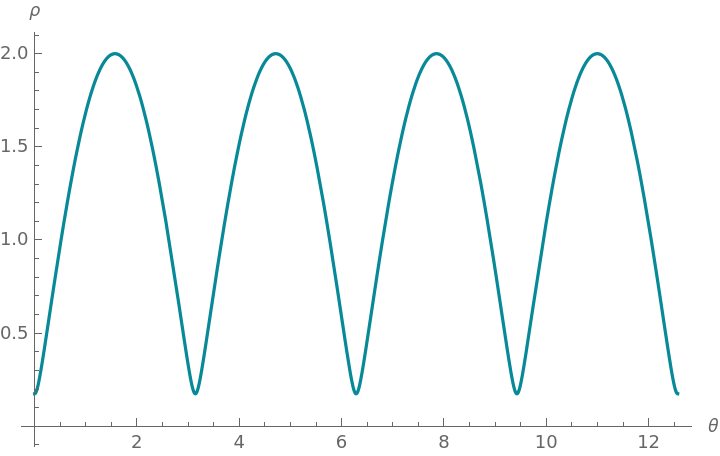
Plot[rho[2,2Pi85/360,θ,0.1/0.6],{θ,0,4Pi},AxesLabel{θ,ρ}]
Out[]=
| | z1>z2 | z1<z2 | ||
Stage | Condition | A 1 | A 1 | A 1 | A 1 |
Withouteclipse | ρ≥ r 1 r 2 | π 2 r 1 | π 2 r 2 | π 2 r 1 | π 2 r 2 |
Partialeclipse | r 1 r 2 r 1 r 2 | π 2 r 1 | π 2 r 2 | π 2 r 1 | π 2 r 2 |
Totalorannular | ρ≤ r 1 r 2 | π 2 r 1 | 0 | π 2 r 1 2 r 2 | π 2 r 2 |
Now we are going to include all the criteria described earlier in the function area[R, i, m2/m1, r1, r2, l1, l2, θ], where: and . The function returns the area that the observer will measure.
m2>m1
r1>r2
Without eclipse: When :
ρ≥+
r
1
r
2
In[]:=
area[R_,i_,q_,r1_,r2_,l1_,l2_,θ_]:=Module[{A1,A2},{A1,A2}={Pir1^2,Pir2^2};l1A1/r1^2+l2A2/r2^2]/;rho[R,i,θ,q]≥r1+r2
Partial eclipse: When +>ρ>-:
r
1
r
2
r
1
r
2
◼
We first calculate ΔA1 and ΔA2
In[]:=
ΔA1[R_,i_,q_,r1_,r2_,θ_]:=Module{ϕ1,ρ,phi,phi1},phi1=LastSolve+-2r1ρCos,phi/.ρ->rho[R,i,θ,q][[1,2]];(ϕ1-Sin[ϕ1])/.ϕ1phi1;ΔA2[R_,i_,q_,r1_,r2_,θ_]:=Module{ϕ2,ρ,phi,phi1},phi1=LastSolve+-2r2ρCos,phi/.ρ->rho[R,i,θ,q][[1,2]];(ϕ2-Sin[ϕ2])/.ϕ2phi1;
2
r2
2
r1
2
ρ
phi
2
1
2
2
r1
2
r1
2
r2
2
ρ
phi
2
1
2
2
r2
◼
In this type of eclipse, for : and while for : and .
z1>z2
A1=π
2
r
1
A2=π-ΔA1-ΔA2
2
r
2
z1<z2
A1=π-ΔA1-ΔA2
2
r
1
A2=π
2
r
2
In[]:=
area[R_,i_,q_,r1_,r2_,l1_,l2_,θ_]:=Module{z1,z2,a1,a2,A1,A2},z1=;z2=;a1=ΔA1[R,i,q,r1,r2,θ];a2=ΔA2[R,i,q,r1,r2,θ];{A1,A2}=If[z1>z2,{Pir1^2,Pir2^2-a1-a2},{Pir1^2-a1-a2,Pir2^2}];l1A1r1^2+l2A2r2^2/;r1+r2>rho[R,i,θ,q]>r1-r2
-RCos[θ]Sin[i]
1+
1
q
RCos[θ]Sin[i]
1+q
Totalorannulareclipse:Whenρ≤-:
r
1
r
2
◼
When r1 > r2 one of the stars will be directly in front of the other one, interposing it. Then a total eclipse will happen if with and , or an annular one will occur if with and .
z1>z2
A1=π
2
r
1
A2=0
z1<z2
A1'=A1-A2
A2'=A2
In[]:=
area[R_,i_,q_,r1_,r2_,l1_,l2_,θ_]:=Module{z1,z2,A1,A2},z1=;z2=;{A1,A2}=If[z1>z2,{Pir1^2,0},{Pir1^2-Pir2^2,Pir2^2}];l1A1r1^2+l2A2r2^2/;rho[R,i,θ,q]≤r1-r2
-RCos[θ]Sin[i]
1+
1
q
RCos[θ]Sin[i]
1+q
Figure
0
.2
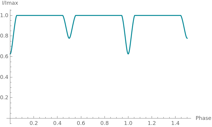
Light curve.Example: With R = 2, i = 85º, m1 = 0.6, m2 = 0.1, R1 = 0.4, R2 = 0.3, l1 = 0.6, l2 = 0.2, we’d like to show I/Imax.
◼
We first calculate Imax.
In[]:=
max=NMaximize[area[2,2Pi85/360,0.1/0.6,0.4,0.3,0.6,0.2,θ],{θ,0,2Pi}][[1]]//Quiet
Out[]=
2.51327
◼
Then we display I/Imax.
In[]:=
Plot[area[2,85Degree,0.1/0.6,0.4,0.3,0.6,0.2,2Piθ]/max,{θ,0,1.5},AxesLabel{"Phase","I/Imax"},AxesOrigin{0,0}]//Quiet
Out[]=
9 Nuclei and Radiations
9
Nuclei and Radiations Application: Modeling the Evolution of a Chain of Isotopes over Time
Application: Modeling the Evolution of a Chain of Isotopes over Time
A radioactive decay chain can be considered as a system of compartments in which the flow is one-directional, as shown in the figure below. This is an example of what is known in compartment modeling as a catenary model.
Graphics[Circle[{0,0},0.5],Text["1",{0,0},{0,0}],Text["",{1.75,.4},{0,0}],Arrow[{{0.5,0},{3,0}}], Circle[{3.5,0},0.5],Text["2",{3.5,0},{0,0}],Circle[{7,0},0.5],Text["3",{7,0},{0,0}],Arrow[{{4,0},{6.5,0}}],Text["",{5.25,.4},{0,0}],{Dashed,Arrow[{{7.5,0},{10.5,0}}]},Text["",{9,.4},{0,0}],AspectRatioAutomatic,AxesNone]
λ
1
λ
2
λ
i

The first circle represents the first isotope in the chain, with a decay constant , the second circle refers to the next isotope, with a decay constant , and so on.
λ
1
λ
2
Let’s consider the case of a chain of 3 isotopes, with (t), (t), and (t) the quantities present of each one at time t, satisfying the following set of differential equations:
q
1
q
2
q
3
q
1
λ
1
q
1
q
2
λ
1
q
1
λ
2
q
2
q
3
λ
2
q
2
λ
3
q
3
◼
As an initial condition let’s assume that at there’s a quantity (atoms, gm, Bq) of isotope 1 in compartment 1 and nothing in the rest. This means: , then:
t=0
q1[0]=b1
q2[0]=q3[0]=0
In[]:=
eq=DSolve[{q1'[t]-λ1q1[t],q2'[t]λ1q1[t]-λ2q2[t],q3'[t]λ2q2[t]-λ3q3[t],q1[0]b1,q2[0]0,q3[0]0},{q1[t],q2[t],q3[t]},t];
◼
The retention in compartments 1, 2, and 3 is given by:
In[]:=
{q1[t_],q2[t_],q3[t_]}={q1[t],q2[t],q3[t]}/.eq[[1]]//Simplify
Out[]=
b1,-,
-tλ1
b1(-)λ1
-tλ1
-tλ2
λ1-λ2
b1λ1λ2((λ1-λ2)+(λ2-λ3)+(-λ1+λ3))
-t(λ1+λ2+λ3)
t(λ1+λ2)
t(λ2+λ3)
t(λ1+λ3)
(λ1-λ2)(λ1-λ3)(λ2-λ3)
Following the same approach, the previous equation can be extended for n daughter isotopes:
(t)=-,withinitialconditions:(t)=,(0)=...=(0)=0
q
n
b
1
n-1
∏
j=1
λ
j
n
∑
j=1
-t
λ
j
n
∏
p=1,p≠j
λ
p
λ
j
q
1
b
1
q
2
q
n
This equation is known as Bateman’s equation, in honor of the mathematician who first published it.
◼
We can type the equation as follows:
Radiation Attenuation
Radiation Attenuation
◼
One way to reduce radiation exposure is through the use of shielding. For example, the thickness of a water layer needed to reduce photon radiation by a tenth is:
◼
In the design of radiation protection products it is important to take into account the mass attenuation coefficients of the materials used. This attenuation depends on the incident particles (protons, alpha, protons, electrons, neutrons) and their energy. Here we compare the mass attenuation coefficient for various substances and energies:
◼
To accurately estimate absorbed doses, we measure the amount of the energy deposited in human tissues. The example below shows the stopping power changes, dE/dx, for an alpha particle emitted from U234 as it travels through biological tissue:
Tsunamis
Tsunamis
We can model very complex natural phenomena. The following demonstration simulates a tsunami using the following system of partial differential equations:
◼
A more realistic simulation is available at:
About Advanced Calculus
Symbolic & Numeric Calculus: http://www.wolfram.com/language/11/symbolic-and-numeric-calculus/
Differential Eigensystems: http://www.wolfram.com/language/11/differential-eigensystems/
Algebra and Number Theory: http://www.wolfram.com/language/11/algebra-and-number-theory/
Partial Differential Equations: http://www.wolfram.com/language/11/partial-differential-equations/
Biokmod: Applications to ICRP Models
Biokmod: Applications to ICRP Models
In this section we’re going to learn more about Biokmod, a Mathematica toolbox developed by the author for modeling biokinetic systems that consists of the following:
(i) A package (Sysmodel) to solve systems of ordinary linear differential equations (SOLDE) with special applications to compartmental and physiological models; (ii) A package for fitting data that can be used to fit transfer rates using experimental data; (iii) A package for optimal design; (iv) Some packages for solving the current ICRP models specially the calculations related to internal doses and bioassay data assessments.
The tutorials included cover: (i) Compartmental and physiological modeling (linear and nonlinear), (ii) Random intakes in occupational exposures and their implications in bioassays, (iii) Analytical methods to evaluate the uncertainties associated with biokinetic model parameters, (iv) Nonlinear regression techniques for bioassay data fitting, (v) Optimal design for bioassay programs.
The tutorials included cover: (i) Compartmental and physiological modeling (linear and nonlinear), (ii) Random intakes in occupational exposures and their implications in bioassays, (iii) Analytical methods to evaluate the uncertainties associated with biokinetic model parameters, (iv) Nonlinear regression techniques for bioassay data fitting, (v) Optimal design for bioassay programs.
The toolbox can be downloaded from: http://diarium.usal.es/guillermo/biokmod/. To install: Extract the file "biokmodXX.zip" with a zip utility (e.g., Winzip). It will create a folder called Biokmod. Copy it to the AddOns\Applications directory in the Mathematica installation folder ($InstallationDirectory).
BIOKMOD can be run in the web: http://oed.usal.es/webMathematica/Biokmod/
Biokmod includes the ICRP models. The ICRP or International Commission on Radiological Protection (http://www.icrp.org) is an independent international organization devoted to preventing the effects associated with exposure to ionizing radiation, and to protect the environment. The ICRP, among other things, publishes models for analyzing the evolution of radioactive particles in the human body and the environment.
All ICRP 66 and 78 models can be represented by compartmental systems with constant coefficients. The generic model used by ICRP 66 and 78 is shown in the below Figure: The particles are deposited in some compartments of the Respiratory Tract (RT). From the RT, the flow goes to the ST (Stomach) or to B (Blood). “Rest of Body” represents the systemic compartments. The detailed flow diagram is specific to each kind of element. The dashed arrows indicate the direction of the flow, depending on the characteristics of the element. The particles are eliminated through fecal or urine excretion. The disintegration can be considered the output from each compartment to the environment; it is given by the disintegration constant of the isotope. This model has been modified by ICRP 130 , but it has not been yet, as of December 2016, included in BIOKMOD. However, the package Sysmodel can be used to solve the models described in the ICRP 130.
The generic ICRP 66 and 78 models applied to the intake of particles by inhalation.
According to it, the human body can be divided in three systems:
c) Systemic compartments: They are specific to an element or groups of elements (ICRP 2001). ICRP 78 (1997) establishes three generic groups: (i) hydrogen, cobalt, ruthenium, cesium, and californium, (ii) strontium, radium, and uranium and (iii) thorium, neptunium, plutonium, americium, and curium. For other elements not included in ICRP 78, the ICRP 30 model applies and they have the same generalized compartmental model as group (i). The same model is used for all the elements of each group although some parameters would change depending on the element. From a mathematical point of view, we can establish two groups: a) Elements whose biokinetic models do not involve recycling, this includes the group (i) and elements where ICRP 30 is still applicable, and b) elements whose biokinetic models involve recycling, this includes group (ii) and (iii).
◼
We will use several packages included in the toolbox. Note that when launching Doses, other packages are also loaded:
The output shows the graphical representations. However, other types of output are available such as retention functions for each compartment or the number of disintegrations accumulated in each compartment.
In this example we assume an exponential input, with t in days, of Iodine–131 by a continuous injection (through a drip):
◼
The total amount injected, in Bq, is given by:
◼
The instruction below returns the retention function for a typical bioassay:
For those readers interested in learning more about the BiokdataReport[...] function, there’s additional information in the BiokMod help files.
The retention function for multiple constant inputs is given by:
The previous equation is the one used by the Biokmod function:
Example: A person is subjected to a medical treatment that consists of a perfusion into the blood of 10 kBq of I–131 every 5 days for 2 hours (or 1/12 day) for 20 days. We would like to know the amount retained in the thyroid function over this period of time.
◼
The unit impulse response can be obtained with the command below (we use the function CompartNumbers to know what compartment number is associated with Thyroid):
◼
Next, we apply the function to the multiple inputs and visualize the results:
A frequent problem in internal dosimetry is how to estimate the quantity of a certain element absorbed from bioassays. This problem is the reverse of what we’ve discussed so far. Let’s see how to solve it with an example.
Example: As a result of the Chernobyl accident (April 26, 1986), a 39 year old civilian male weighing 80 kg was exposed to a continuous and unknown ingestion of Cs–137 (data from Ansoborlo et al., 2003).
◼
The measurements related to the evolution of the element retention over time in his body are given below: {time after the accident (d), activity (Bq)}:
◼
The function below computes the overall retention for an acute intake, "1" , of Cs–137 at t = 0:
◼
We can see that the retention was increasing until T. Assuming that it happened until that time and then stopped, we can fit the experimental data, taking into consideration both periods, before and after T.
In[]:=
model2[t1_?NumericQ, p_?NumericQ, tt_?NumericQ] := p qConstant[1,{qWbCs137[t],t}, t1, tt]
◼
To estimate the best fit for the intake I in Bq/day, and the period T, in days:
◼
Then, the accumulated intake is:
◼
The quality of the fit is shown in the plot below:
Doses
Doses
Exposure to ionizing radiations may result in radiological risk. To estimate such risk, the concept of dose, measured in Sieverts (Sv, mSv), was introduced.
Almost all of the radiation that we receive on a regular basis comes from either nature or medical tests. The average annual exposure is 2.4 mSv/year per person. However, this number varies widely, ranging from 2 to 10 mSv/year, depending on the place and costumes of the specific individuals (types of food consumed, smoking habits and dwelling). There are even regions, such as Kerala in India, that amply exceed this range. As a precaution, we assume that any dose carries the risk of producing undesirable biological effects; that the relationship between the risk and the dose is linear (that is, double dose double risk); and that any dose, no matter how small, carries a risk. These criteria are used as a precaution since it's not possible to know if an effect (e.g., a certain type of cancer) is attributable to the radiations or has a different cause. For example: the linear hypothesis implies that a dose of 100 mSv may result in a 0.1% increase in the risk of cancer, a change not big enough to clearly identify the dose as the cause of the disease.
Radiation exposure can originate from either irradiation (i.e. X-rays) or assimilation (inhalation, ingestion or injection) of radioactive particles by the human body. In the first case, the exposure stops when we move away from the radiation source (for example: a radiography). However, if we assimilate the radioactive source (for example: by ingestion or injection of a radioactive isotope) the exposure continues as long as the radioactive substance remains in our body. Next, we describe how to calculate the dose in this last case.
Example: An adult person receives an injection of 0.01 μg of I–131. What would be the thyroid effective dose?
The previous result indicates the extraordinary radioactive activity of such a small amount of Iodine–131, an isotope widely used in oncological treatments and medical research. Because of that, patients being treated with the isotope need to take certain precautions if they live with other people.
The effective dose is 1 Sv and the equivalent dose in the Thyroid is 20.0 Sv, a very high dose.
◼
In the previous section, we found that a male was exposed to an ingestion of 13,132.9 Bq of Cs–137. In term of doses, this is equivalent to:
This value is negligible compared to the dose received from a typical medical treatment.
Control Systems
Control Systems
Internal Ratings-Based (IRB) Approach
Internal Ratings-Based (IRB) Approach
The key cornerstone of prudential regulation of banks (and financial institutions in general) is to ensure that each bank holds sufficient equity capital to absorb unexpected losses, that is, the materialization of financial risks, mainly market (price), credit, and operational risks.
The example below, Basel II Capital Adequacy: Internal Ratings-Based (IRB) Approach, by Poomjai Nacaskul, shows how to calculate, using the Internal Ratings-Based approach, the minimum amount of capital that a bank should keep following the standards defined by the Basel II regulatory framework on bank capital adequacy.
◼
To facilitate the understanding of the example, we also include the code:
To learn more about financial modeling and risk management using Mathematica, Igor Hlivka has created several excellent example notebooks. You can find them in:
Application: Analyzing Enriched Uranium
Application: Analyzing Enriched Uranium
A key aspect in the operation of nuclear power plants is the cost of the fuel. Virtually all nuclear reactors use uranium as their main source of energy input. The minerals containing it are widely distributed in nature, but profitable deposits under current economic conditions are concentrated in a limited number of countries. According to estimates, these deposits will last for another 70 to 80 years which reduces the amount of money invested in finding new sources. Fast reactors that reuse uranium would extend the availability of the nuclear fuel to thousands of years. However, the cost and the immaturity of the technology don’t justify the development of this type of reactor for the time being. Nevertheless, the current ones, although inefficiently, can reuse part of the spent fuel. Some power plants already do that.
◼
Uranium found in nature mostly consists of three isotopes. The command below displays their respective abundance (fraction of atoms of an isotope in the element). We can see that almost everything is either U238 or U235:
Most nuclear reactors use uranium enriched in the U–235 isotope. The proportion of this isotope in heavy metals can reach up to 5%. The process to enrich uranium consists of two steps: turning natural uranium into gas (UF6) and then putting the gas into centrifuge tubes (there are other enrichment techniques but this one is the most commonly used). The centrifuge tubes are cylinders that spin at very high speeds pulling the heavier U–238 into the walls of the cylinder and leaving the lighter U–235 closer to the center where it can be sucked out. The result is the extraction of uranium with a higher proportion of U–235 than the one found in nature.
(Log is the natural logarithm, that is, in base )
The previous equation doesn’t refer to the real energy consumption that depends on the technology used. It’s based on the thermodynamical notion of consumption and there’s an agreement to use it regardless of the real consumption.
◼
In the next example we calculate the feed and SWU needed to obtain 5% enriched uranium with a tail of 0.3%.
◼
For a given tail, in the command below we use 0.2%, the function calculates the SWU required for 1 kgU with enrichment enr:
◼
We fit the previous function to a line in the range enr 1.0% - 3.5%.
◼
Now we compare the exact calculation and its numerical approximation. We can see that both lines, although close to each other, are different.
For the uranium buyer, the setting of the tail is very important and that choice will be determined by the cost of the feed and the SWU.
The enriched uranium cost can be computed using the following expression:
◼
The next function calculates the price of 1 kgU for a given tail, enrichment level and feed and SWU prices:
We can get the spot feed (natural UF6 in kgU) and SWU prices from http://www.uxc.com/review/UxCPrices.aspx. If we open the link (registration required), the information will be inside the table: Ux Month-End Spot Prices as of MM, YYYY.