ABSTRACT (original article): The classical solution to the Helmholtz wave equation in spherical coordinates is well known and has found many important applications in wave propagation, scattering, and imaging in optics and acoustics. The separable solution is comprised of spherical Bessel functions in the radial direction and spherical harmonics in the angular directions. The nature of the spherical Bessel functions includes a long asymptotic oscillatory tail at large radii, not conducive to applications where a tight concentration of wave amplitude around a ring is desired, for example in toroidal configurations. However, we have found that certain practical bandpass spectral shapes, centered around a peak frequency, can create a superposition of spherical Bessel functions that effectively concentrate the wave amplitude around a defined ring at the time instant of coherent addition, avoiding the long tail asymptotic oscillations of the single frequency solution. Theoretical solutions are shown for different bandpass spectra applied to the spherical Bessel functions, along with numerical solutions of transient wave propagation using practical hemispherical source shapes. These findings introduce a framework by which ring or toroidal concentrated waves can be produced with a simple bandpass superposition applied to hemispherical source shapes and with reference to the classical solutions in spherical coordinates. CITATION (original article): Kevin J. Parker, Miguel A. Alonso (2024), The concentrated toroidal wave, arXiv:2410.11700. https://doi.org/10.48550/arXiv.2410.11700
In wave propagation applications, integrations across sources and integrations across frequencies are frequently required to specify the wave propagation patterns in free space. For complicated problems, numerical integrations are used where analytical solutions are unavailable. This notebook contains examples of broadband pulse propagations from hemispherical sources, which can be constructed advantageously to produce very concentrated toroidal shaped intensity patterns. We used the ParametricRegion definition to conveniently describe hemispherical source regions in a 3D space. Once defined in natural spherical coordinates, this ParametricRegion could be used to define the surface integration across the active source, in Cartesian coordinates. We then used NIntegrate to add up all the source terms, both from the hemispherical shaped source and across all frequencies in the active bandwidth.
The ParametricRegion definition was also helpful for graphics commands, including SliceDensityPlot3D and other 2D and 3D plotting functions. A more detailed description of the theoretical basis, and useful results of this investigation are found in: https://arxiv.org/abs/2410.11700
The ParametricRegion definition was also helpful for graphics commands, including SliceDensityPlot3D and other 2D and 3D plotting functions. A more detailed description of the theoretical basis, and useful results of this investigation are found in: https://arxiv.org/abs/2410.11700
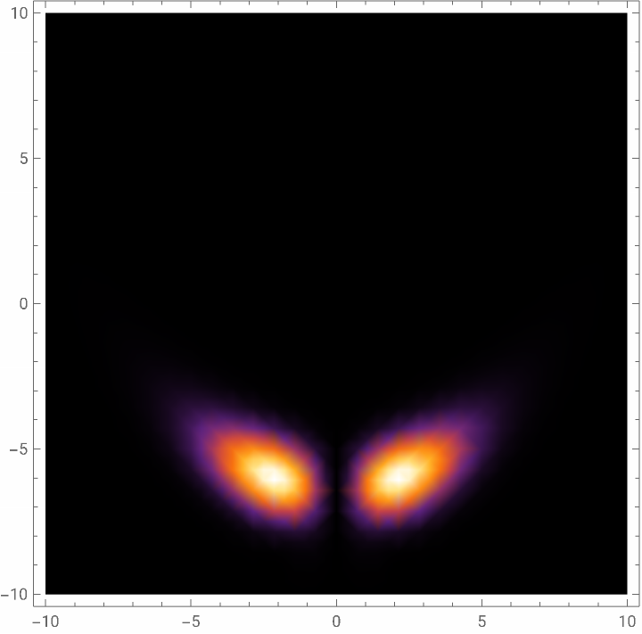
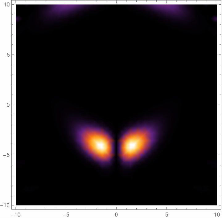
Samples of calculations used in "Concentrated Spherical Harmonics" paper by Parker and Alonso, by integrating over frequency or wavenumber to create a broadband pulse. The source is assumed to be active on a sphere of radius 8 Pi, all units normalized, speed c = 1 distance/time units .
Calculate the time / phase shift on the source that is a semi-hemisphere shell we call the "lemon wedge" shape
Y4b is Cartesian form of the Y 4 4 Spherical Harmonic shape
Note: many graphics parameters used in publication are downgraded herein for more rapid completion
Y4b is Cartesian form of the Y 4 4 Spherical Harmonic shape
Note: many graphics parameters used in publication are downgraded herein for more rapid completion
In[]:=
reg4c=ParametricRegion[{8*Pi*Sin[th]Cos[phi],8*Pi*Sin[th]Sin[phi],8*Pi*Cos[th]},{{th,0,Pi/1},{phi,Pi/4,3Pi/4}}];
zo=0.01;R=Sqrt[(x-xo)^2+(y-yo)^2+(z-zo)^2];f=Sqrt[x^2+y^2+z^2];kgf=Exp[I*k*R]/R;Y4b=
4x(x-y)y(x+y)
2
(++)
2
x
2
y
2
z
Out[]=
4x(x-y)y(x+y)
2
(++)
2
x
2
y
2
z
Below, source and pattern of source strength, then intensity at zero reference time in the equatorial plane
SliceDensityPlot3D[(Abs[Y4b*f])^2,reg4c,{x,-8*Pi,8*Pi},{y,-10*Pi,10*Pi},{z,-8*Pi,8*Pi},ImageSizeSmall]
Out[]=

In[]:=
DensityPlot[Abs[(NIntegrate[(Sum[Exp[I*k*0](k^6Exp[-(1/4)k^2])kgf,{k,0.6,8.2,0.2}])*Y4b,{x,y,z}∈reg4c,MaxPoints6220,MaxRecursion12,PrecisionGoal2,AccuracyGoal2])]^2,{xo,-10,10},{yo,-10,10},PlotRangeAll,PerformanceGoal"Quality",ColorFunction"SunsetColors"]
In[]:=
DensityPlot[Abs[(NIntegrate[(Sum[Exp[I*k*2](k^6Exp[-(1/4)k^2])kgf,{k,0.6,8.2,0.4}])*Y4b,{x,y,z}∈reg4c,MaxPoints6220,MaxRecursion2,PrecisionGoal2,AccuracyGoal2])]^2,{xo,-10,10},{yo,-10,10},PlotRangeAll,PerformanceGoal"Quality",ColorFunction"SunsetColors"]
Out[]=
Y4b=
4x(x-y)y(x+y)
2
(++)
2
x
2
y
2
z
Out[]=
4x(x-y)y(x+y)
2
(++)
2
x
2
y
2
z
In[]:=
reg4b=ParametricRegion[{8*Pi*Sin[th]Cos[phi],8*Pi*Sin[th]Sin[phi],8*Pi*Cos[th]},{{th,Pi/2,Pi/1},{phi,0,2Pi}}];
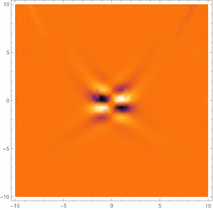
Below, check on the Real part of the wave, plus and minus going through the middle origin.
DensityPlot[Re[(NIntegrate[(Sum[Exp[I*k*6](k^6Exp[-(1/4)k^2])kgf,{k,0.6,8.2,0.4}])*Y4b,{x,y,z}∈reg4c,MaxPoints6220,MaxRecursion2,PrecisionGoal2,AccuracyGoal2])],{xo,-10,10},{yo,-10,10},PlotRangeAll,PerformanceGoal"Quality",ColorFunction"SunsetColors"]
Out[]=
Below, 3D comparison of monochromatic spherical wave, theoretical result.
In[]:=
DensityPlot3DAbsSphericalBesselJ4,++SphericalHarmonicY4,4,ArcTanz,+,ArcTan[x,y]^2,{x,0,14},{y,-14,14},{z,-14,14}
2
x
2
y
2
z
2
x
2
y
Out[]=

CITE THIS NOTEBOOK
CITE THIS NOTEBOOK
The concentrated toroidal wave
by Kevin Parker & Miguel Alonso
Wolfram Community, STAFF PICKS, October 23, 2025
https://community.wolfram.com/groups/-/m/t/3564089
by Kevin Parker & Miguel Alonso
Wolfram Community, STAFF PICKS, October 23, 2025
https://community.wolfram.com/groups/-/m/t/3564089