Transient Cooling of a Composite Two-Dimensional Slab
Transient Cooling of a Composite Two-Dimensional Slab


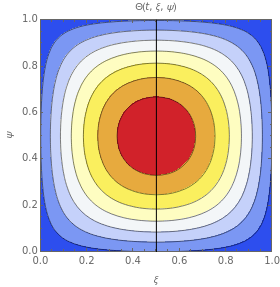
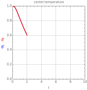
This Demonstration simulates the transient cooling of a composite slab that is suddenly immersed in a cooling bath.
Consider a square slab of side , consisting of two parallel layers in perfect thermal contact, initially at uniform temperature . The slab is immersed at time in a well-stirred, insulated tank containing a fluid at constant temperature .
L=1
T
0
t≥0
T
∞
The heat equation describing this system is:
∂T
∂t
∂T
∂
2
x
∂T
∂
2
y
with
k+h(T-)=0
∂T
∂x
T
∞
x=0
x=L
k+h(T-)=0
∂T
∂y
T
∞
y=0
y=L
T(0,x,y)=
T
0
where and are the space coordinates, (), is the thermal diffusivity (/sec), is the thermal conductivity () and is the heat transfer coefficient between the slab and the surrounding fluid ().
x
y
cm
α
2
cm
k
W/cm·K
h
W·/K
2
cm
To solve this problem, it is convenient to introduce the following dimensionless variables:
Θ=-
T-
T
∞
T
0
T
∞
ξ=
x
L
and
ψ=
y
L
∂Θ
∂t
∂Θ
∂
2
ξ
∂Θ
∂
2
ψ
∂Θ
∂ξ
ξ=0
ξ=1
∂Θ
∂ψ
ξ=0
ξ=1
Θ(0,ξ,ψ)=1
with
α=
|
and
Bi=
|
where is the Biot number, the ratio of internal resistance to conductive heat transfer in the slab to the external resistance of convective heat transfer from the slab to the surrounding fluid; is the dimensionless line of separation between the two layers; and the subscripts and refer to thermal properties of the layers and , respectively.
Bi=
hL
k
λ
1
2
x≤λ
x>λ
External Links
External Links
Permanent Citation
Permanent Citation
Clay Gruesbeck
"Transient Cooling of a Composite Two-Dimensional Slab"
http://demonstrations.wolfram.com/TransientCoolingOfACompositeTwoDimensionalSlab/
Wolfram Demonstrations Project
Published: July 26, 2018