Consider a binary mixture composed of -hexane and -octane. First, we reproduce the enthalpy versus composition diagram at 101.325 kPa (show below).
Then, we plot the same diagram using our own data. Finally, we superimpose both data sets.
n
n
Then, we plot the same diagram using our own data. Finally, we superimpose both data sets.
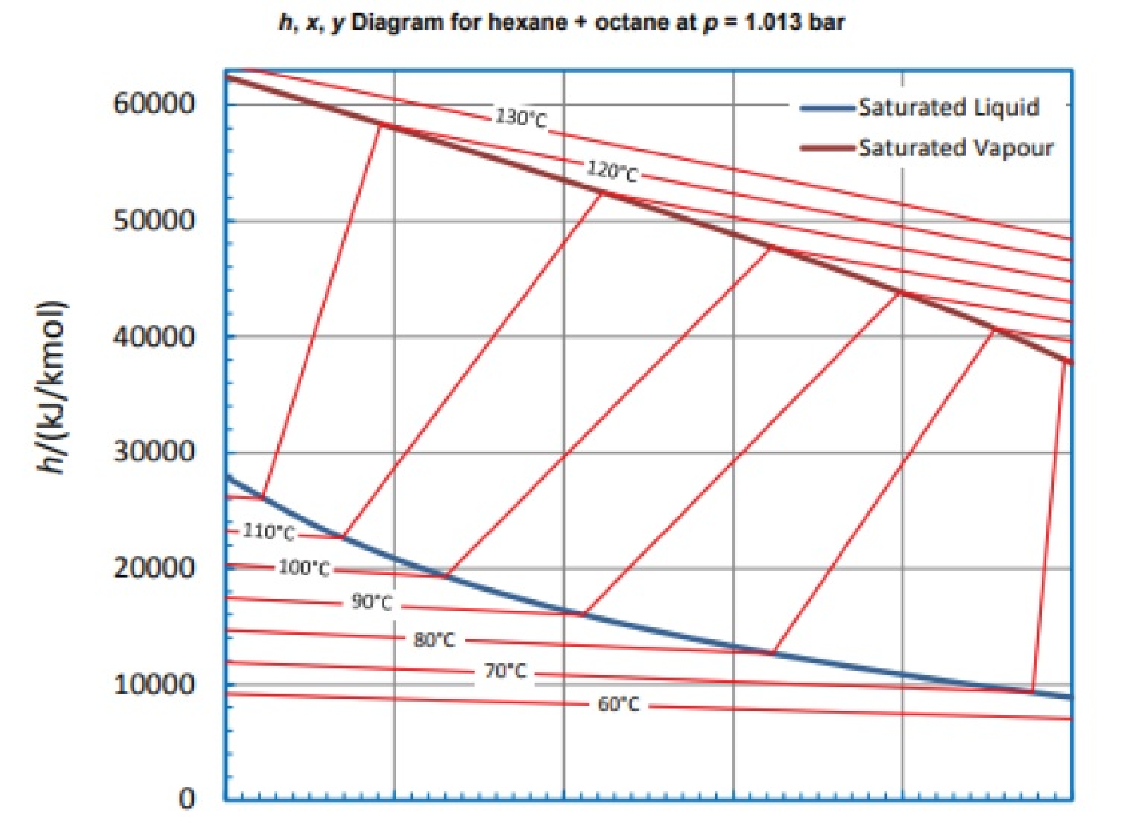
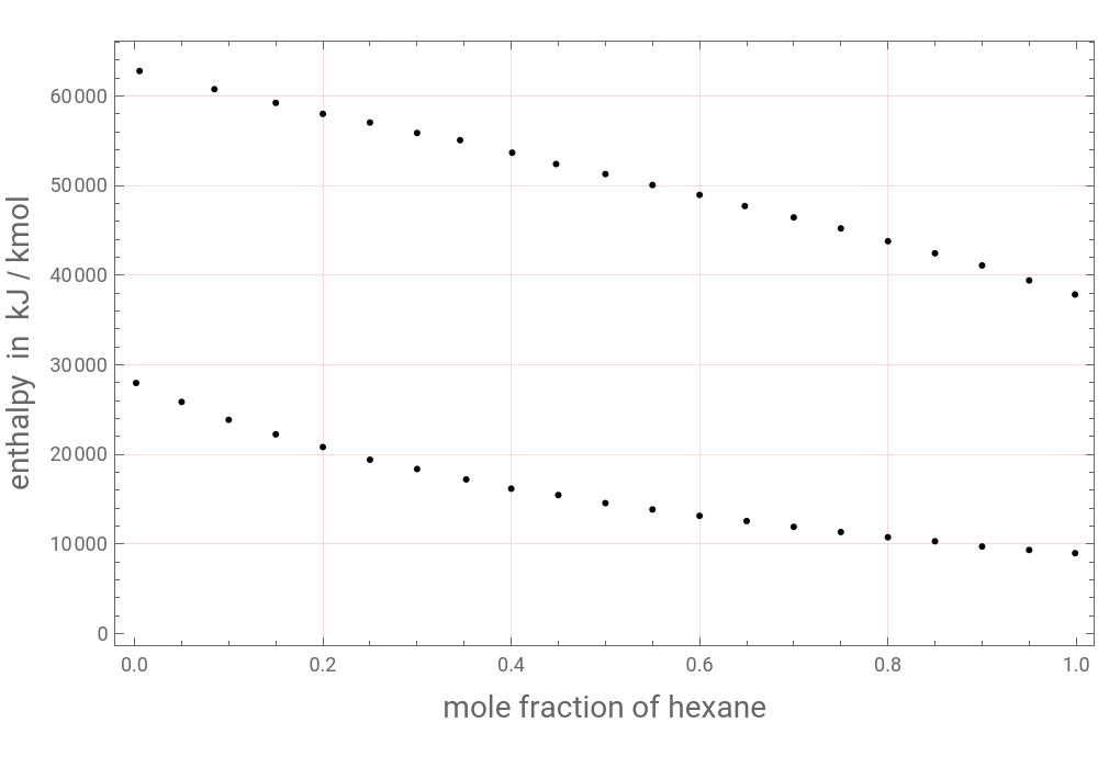
Using the digitized data from the Figure above, we construct the h-x and H-y diagram.
In[]:=
data={{0.05,25862.8},{0.1,23862.3},{0.15,59225.6},{0.15,22249.},{0.2,57999.5},{0.2,20829.3},{0.25,57031.5},{0.25,19409.6},{0.3,55870.},{0.3,18377.1},{0.4,16183.1},{0.45,15473.2},{0.5,51288.2},{0.5,14569.8},{0.55,50062.1},{0.55,13859.9},{0.6,48965.1},{0.6,13150.1},{0.65,12569.3},{0.7,46448.4},{0.7,11924.},{0.75,45222.3},{0.75,11343.2},{0.8,10762.4},{0.85,42447.4},{0.85,10310.7},{0.9,41092.3},{0.9,9729.91},{0.95,39414.4},{0.95,9342.72},{0.800096,43797.5},{0.352197,17215.2},{0.447652,52405.1},{0.345729,55063.3},{0.00534361,62784.8},{0.001606,27974.7},{0.998781,8987.34},{0.998715,37848.1},{0.0848116,60759.5},{0.401012,53670.9},{0.648074,47721.5}};
In[]:=
P1=ListPlot[{data},FrameTrue,FrameLabel{Style["mole fraction of hexane",14],Style["enthalpy in kJ / kmol",14]},GridLinesStyleDirective[LightRed],GridLinesAutomatic,ImageSize{500,350},PlotStyle{{Darker@Red,Thick},{Darker@Blue,Thick}}]
Out[]=
Generating our own data with the help of Aspen-Hysys®
Total pressure in bar
In[]:=
P=1.01325;
Antoine Constants and equation for hexane and octane
In[]:=
Psat1[temp_]:=10^4.00266-;(*hexane*)Psat2[temp_]:=10^4.04867-;(*octane*)
1171.53
temp+224.216
1355.126
temp+209.367
Normal boiling temperatures in °C
In[]:=
FindRoot[Psat1[T]P,{T,60}]
Out[]=
{T68.8905}
In[]:=
FindRoot[Psat2[T]P,{T,60}]
Out[]=
{T125.815}
Computing VLE data for the binary system: Ethanol and Water as well as h-x and H-y data
In[]:=
i=0;While[i<1001,{xa=i0.001,sol=FindRoot[Psat1[T]xa+Psat2[T](1-xa)P,{T,77,78}];xe[i]=xa,ye[i]=Psat1[T]xa/P/.sol,Te[i]=273.15+T/.sol,i++}];Tbl1=Table[{xe[i],Te[i]-273.15},{i,0,1000}];Tbl2=Table[{ye[i],Te[i]-273.15},{i,0,1000}];Tbl3=Table[{xe[i],ye[i]},{i,0,1000}];Tx=Interpolation[Tbl1,InterpolationOrder1];(*bubbletemperaturein°C*)Ty=Interpolation[Tbl2,InterpolationOrder1];(*dewtemperaturein°C*)xy=Interpolation[Tbl3,InterpolationOrder1];(*VLEdata*)(*purecomponententhalpies-referencestates:h1=h2=0at25°Cand101.325kPa*)A=(0.0+198.2T-0.1933T^2+4.21010^-004T^3-1.62410^-012T^4)/.T(25+273.15);hl1=0.0+198.2T-0.1933T^2+4.21010^-004T^3-1.62410^-012T^4-A;B=(0.0+241.5T-0.1389T^2+3.5410^-004T^3-8.61210^-013T^4)/.T(25+273.15);hl2=0.0+241.5T-0.1389T^2+3.5410^-004T^3-8.61210^-013T^4-B;Hv1=43550+179.2T-0.3160T^2+7.21210^-004T^3-4.34710^-007T^4-A;Hv2=54680+220.1T-0.2676T^2+6.31410^-004T^3-3.51110^-007T^4-B;(*mixtureenthalpies*)Hvhysys[y_]:=(yHv1+(1-y)Hv2)/.T(Ty[y]+273.15);hlhysys[x_]:=(xhl1+(1-x)hl2)/.T(Tx[x]+273.15);
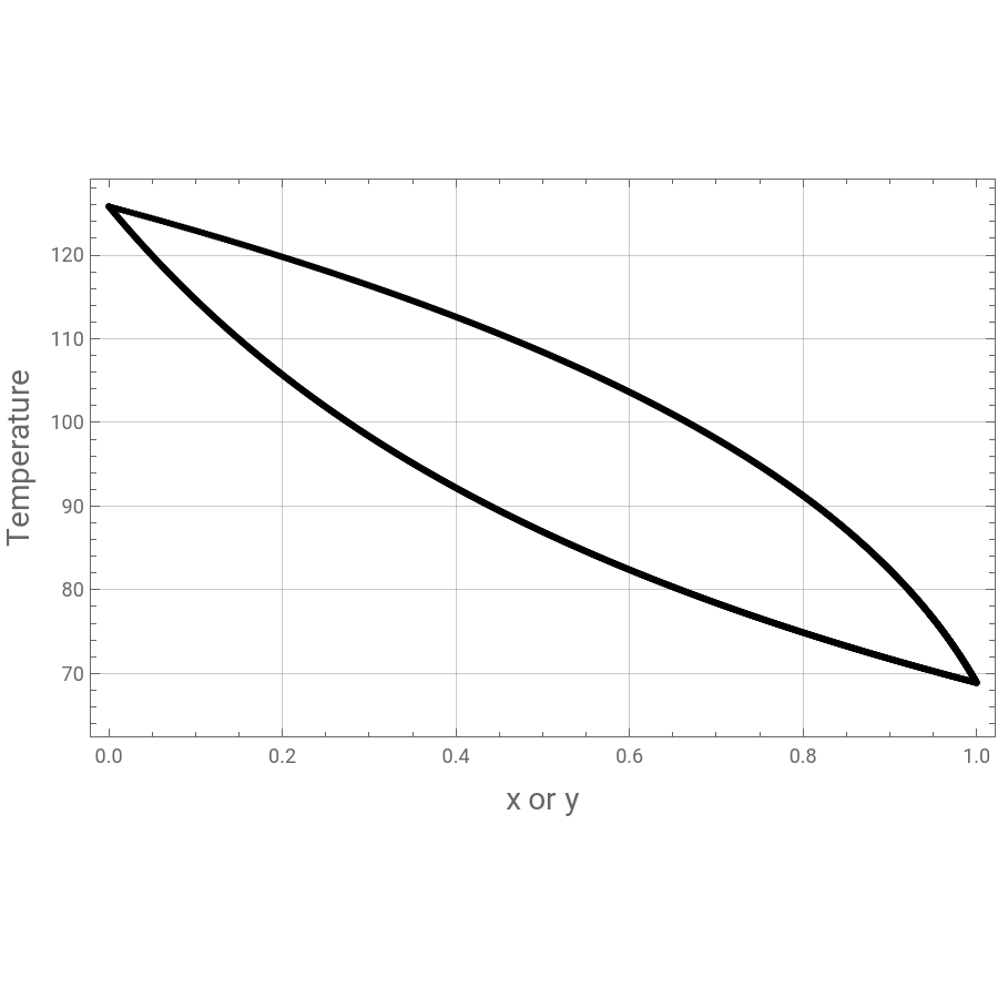
Plotting VLE data for the binary system (hexane/octane) as well as h-x and H-y data
In[]:=
ListPlot[{Tbl1,Tbl2},FrameTrue,GridLinesAutomatic,ImageSize450{1,1},FrameLabel{Style["x or y",14],Style["Temperature",14]}]
Out[]=
In[]:=
P2=Plot[{hlhysys[x],Hvhysys[x]},{x,0,1},FrameTrue,FrameLabel{Style["mole fraction of hexane",14],Style["enthalpy kJ / kmole",14]},GridLinesAutomatic,ImageSize{600,350},PlotStyleThick,PlotRange{{0,1},All},AxesOrigin{0,3000}]
Out[]=
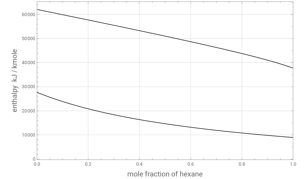
Comparison by superposing the two diagrams
Adding a few tie lines (shown in green) to the Enthalpy - Composition diagram
tie lines from the open literature
Our calculated tie lines
CITE THIS NOTEBOOK
CITE THIS NOTEBOOK
Enthalpy versus Composition Diagram for n-Hexane/n-Octane at 101.325 kPa
by Housam Binous and Ahmed Bellagi
Wolfram Community, STAFF PICKS, January 13, 2024
https://community.wolfram.com/groups/-/m/t/3102743
by Housam Binous and Ahmed Bellagi
Wolfram Community, STAFF PICKS, January 13, 2024
https://community.wolfram.com/groups/-/m/t/3102743