Wolfram Cloud Document

The Wolfram Emerging Leaders Program: High School (WELP:HS) is a remote, semester-long program designed for exceptional graduates from the Wolfram High School Summer Research Program to continue to develop their skills. Students work in a small group over the course of a semester to do either a research-based project or a product development–based project under the guidance of expert mentors. Projects are centered around a topic at the intersection of the group’s interests.

◼

Mariem El-Kady

◼

Hao Wei

One-dimensional cellular automata (CA) provide a minimal model for complex growth from simple rules. In this project, we explore point mutations (single-bit changes in the rule definition) and study how such mutations generate “megafauna”: unusually large or expansive organisms within the CA. By comparing unmutated and mutated automata, we aim to understand how small rule perturbations affect emergent size and structure. Our focus is to construct a mutation environment, measure organism growth, and identify conditions that yield the largest evolving patterns.

Introduction

Cellular automata (CA) are simple computational systems consisting of cells that update based on local rules. Despite their simplicity, Stephen Wolfram’s work—particularly in “A New Kind of Science” and “Foundations of Biological Evolution: More Results & More Surprises”—shows that even 1D binary CA can generate elaborate, lifelike behavior. A rule in a one-dimensional CA specifies how each cell updates based on itself and its two neighbors, producing a space-time pattern when iterated over many steps.

In evolutionary CA studies, a point mutation refers to changing one bit in the 8-bit rule table that defines the automaton. This allows us to explore how minimal changes in the underlying “genetic code” of the rule affect the resulting organism-like pattern. Large, complex structures emerging from such systems are often referred to as megafauna, borrowing from biological terminology to describe unusually large or intricate computational organisms.

Our project investigates how point mutations influence the growth, size, and morphology of CA organisms. Using a baseline rule, we generate an initial pattern from a single seed and then apply mutated versions of the rule to observe how structure changes.

CA Environment Base

We begin by establishing the basic environment for our 1D cellular automaton. The system contains 200 cells arranged linearly, and it will evolve for 50 time steps. We want the system to evolve

In[]:=

numCells=200;numSteps=50;

We’ll work with k=3, r=1 rules first. Thus, our rules are going to have 27 possible digits in base-3.

In[]:=

RulePlot[CellularAutomaton[{0,3}]]

Out[]=

Since we want the last condition to always lead to 0, we can omit this and use a 26-“bit” rule instead.

get27bitRule converts a 26-bit CA rule into a 27-bit CA rule

In[]:=

get27bitRule[prerule_]:=Insert[prerule,0,27]

The initial configuration consists of a single active cell placed exactly at the center of the lattice, with all other cells inactive (“0”).

This standard initial condition allows us to directly compare the spatial growth produced by different rules or mutated versions of the same rule.

In[]:=

initialState = Table[If[i == Floor[numCells/2],2,0],{i,numCells}];

evolveCA converts our rule to decimal for use with Wolfram’s optimized function

In[]:=

evolveCA[init_List, ruleBits_List, steps_Integer] := CellularAutomaton[{FromDigits[get27bitRule[ruleBits], 3], 3}, init, steps]

Here we generate the full space–time evolution for the selected rule and visualize it using ArrayPlot. Black pixels represent active cells and white pixels represent inactive cells. This plot provides a direct view of the organism-like patterns produced by the elementary CA rule before introducing any mutations. Later, mutated rule versions will be visualized similarly, allowing comparison of emergent “megafauna” growth.

An example of evolveCA on the null rule

In[]:=

ArrayPlot[evolveCA[initialState,ConstantArray[0,26],numSteps]]

Out[]=

Mutating rules

Having established the baseline CA environment, we now introduce the evolutionary component of the model. The goal of this section is to simulate how a rule-encoded organism changes when random point mutations are applied, and to measure whether such mutations produce larger or more expansive “organisms” in the CA space-time pattern.

In this system, each rule is represented as a 26-element list rather than the standard 8-bit Wolfram rule. This extended encoding lets us explore a richer evolutionary landscape, where each element can mutate independently to values 0, 1, or 2.

The function pointMutate takes a rule (a list of 26 integers) and generates all possible single-point mutations. For each position in the rule, it creates 26 rule positions can mutate to 2 alternative states.

In[]:=

pointMutate[rule_] := Module[{}, RandomSample[ Flatten[Table[ ReplacePart[rule, x -> Discard[{0, 1, 2}, # == rule[[x]] &][[y]]], {x, 26}, {y, 2}], 1]] ]

An example of pointMutate; finds the 52 possible point mutations for the null rule

In[]:=

pointMutate[ConstantArray[0,26]]

To test whether a mutation leads to a stronger or weaker organism, we need a way to quantify “fitness.”

The function getRuleData evolves the automaton using a given rule and then measures two characteristics: trialLength — how many time steps contain at least one active cell trialWidth — how many spatial positions ever become active across the entire simulationTogether, these numbers estimate how far the CA organism spreads vertically (time) and horizontally (space).

In[]:=

getRuleData[rule_List]:=Module[{trialData=evolveCA[initialState,rule,numSteps],trialLength,trialWidth},trialLength=Length[Select[trialData,AnyTrue[#,Positive]&]];trialWidth=Length[Select[Transpose[trialData],AnyTrue[#,Positive]&]];{trialLength,trialWidth}]

With mutation and measurement functions in place, we now implement the evolutionary selection process. Out of the 52 possible point mutations, the rule with the greatest width but still halting before tick 50 is considered to be the most fit rule. If there is no rule that is both greater than the original rule and halts before tick 50, the program selects a the rule that is the closest to the width of the original rule without continuing past tick 50.

The function testRules evaluates all possible single-point mutations of a parent rule and selects the most promising candidate based on growth metrics.

In[]:=

testRules[startingRule_List]:=Module[{startingRuleData=getRuleData[startingRule],possibleMutations,mutationData,filteredMutationData},possibleMutations=AssociationMap[getRuleData,pointMutate[startingRule]];mutationData=Discard[possibleMutations,#[[1]]>numSteps||#[[2]]<=startingRuleData[[2]]&];filteredMutationData=If[mutationData==<||>,Nearest[Discard[possibleMutations,#[[1]]>=numSteps&][[All,2]],startingRuleData[[2]]],Keys[mutationData]];First[filteredMutationData]]

The selection criteria prioritize mutations that increase spatial width while maintaining viability (not exceeding the simulation time bounds). If no mutation improves spatial extent, the function falls back to selecting the mutation with the largest available width.

Finally, mainSimulation repeatedly applies testRules, building a chain of descendants over many evolutionary steps.
This constructs a full evolutionary trajectory starting from an initial rule, allowing us to observe how rule-space mutations produce progressively larger or more complex organisms.

In[]:=

mainSimulation[startingRule_List, simulatedSteps_Integer] := Module[{}, NestList[testRules, startingRule, simulatedSteps] ]

Let’s run an evolutionary simulation and visualize the progression of CA patterns:

dataNullRule=mainSimulation[ConstantArray[0,26],300];

ParallelTable[ArrayPlot[evolveCA[initialState,x,numSteps],ImageSize->Small],{x,dataNullRule[[;;50]]}]

Out[]=





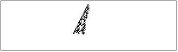
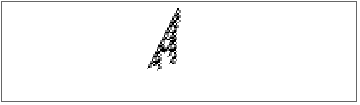
When we mutate the null rule one bit at a time, the CA does not immediately jump into complex behavior. Instead, it produces patterns that expand extremely slowly. A single-bit mutation usually activates only one neighborhood transition, so growth can only occur when that specific neighborhood appears, and the CA must generate it through repeated evolution.

As a result, the width of the organism increases at a very low rate — sometimes less than one cell per 20–50 iterations. This explains why, after 300 steps, many rules appear almost empty except for a thin diagonal line. Although visually minimal, these diagonals actually represent consistent, steady growth: a glider-like structure that expands the organism boundary little by little.

This implies that the mutational landscape near the null rule is dominated by extremely low-growth phenotypes. Complexity and expansion require coordinated changes in multiple rule bits, and point mutations rarely achieve that immediately. Thus, the CA evolves, but it does so through a long period of very slow improvements.

This implication opens a new hypothesis that can be tested: Is a mutation’s state highly affected by its neighbouring environment in cellular automata?

The Effect of Starting Conditions on Evolutionary Progress

Having observed slow evolutionary progress from the null rule, we now test whether different starting conditions affect the discovery of complex “megafauna” patterns. We compare three starting points: the null rule (all zeros), a minimal rule (single active bit), and the all-ones rule (maximum initial activity).

Minimal Rule: Starting with a Single Active Bit

Instead of beginning with complete inactivity, we initialize evolution with a rule containing just one active transition. This provides immediate growth potential while maintaining minimal complexity.

minimalRule is defines with one active transition.

Now, we are running the evolutionary simulation on minimalRule.

Observations from minimal rule evolution:

The rule maintains its initial active bit at position 13 throughout evolution

Additional active bits gradually appear at other positions

State 2 (gray) emerges by generation 4, creating more complex interactions

The pattern shows steady but gradual complexity increase

The patterns show more immediate growth than the null rule, with visible expansion starting from early generations. While still considered slow evolution, the minimal rule demonstrates more promising development than starting from complete inactivity.

The All-Ones Rule

We also test an extreme starting condition: the all-ones rule, where every neighborhood produces an active cell. This represents maximum initial activity.

The error represents an evolutionary dead-end where a population has reached a fitness plateau. Every possible point mutation produces offspring with identical fitness to the parent (200), creating neutral evolution without selective advantage. The algorithm’s selection criterion demands strict improvement (fitness ≤ parent fitness), so all mutations are discarded, leaving no genetic variation for natural selection to act upon.

This mirrors real evolutionary scenarios where:

Local optimum trap: The genotype is trapped at a local fitness peak where all immediate neighbors offer no improvement

Neutral network exhaustion: The population has explored all accessible neutral mutations without finding a path to higher fitness

Selective constraint: The strict “improvement-only” selection pressure eliminates all variation, preventing evolutionary exploration

Thus we conclude that while a general state of inactivity might slow down a rule’s evolution, on contrary a state of excessive activity causes the system to degenerate in a state of “reverse evolution.”

Comparative Analysis

To put everything in perspective, let’s briefly compare the null rule with the minimal rule

The graph reveals two distinct evolutionary paths from different starting conditions. The Null Rule, beginning with complete inactivity, shows quite rapid initial adaptation that quickly plateaus at a moderate fitness level. This represents efficient but limited evolution—it quickly exploits available improvements but then exhausts its adaptive potential, becoming trapped at a local optimum with no path to higher fitness.

In contrast, the Minimal Rule, starting with just one active site, follows a slightly slower, more exploratory trajectory. While its initial progress is more gradual, it ultimately reaches higher fitness peaks and displays semi-periodic adaptive breakthroughs even after apparent stabilization. This demonstrates sustained evolutionary potential through continued exploration of the fitness landscape.

Varying k and its affect on evolution

After exploring evolutionary dynamics in k=3 cellular automata, we investigate how increasing the number of possible states per cell (k) affects evolutionary progress. Does a larger state space accelerate the discovery of complex “megafauna” patterns, or does it create a more challenging search landscape? We extend our framework to k=4 systems, where each cell can be in states {0, 1, 2, 3}, requiring adaptation of all evolutionary components.

k=4 Rule Encoding and Evolution

For k=4 cellular automata, we have 4³ = 64 possible neighborhood patterns. Our rule encoding requires 63 bits (converted to 64 bits for compatibility with Wolfram’s CellularAutomaton function).

get64bitRule converts a 63-bit CA rule into a 64-bit CA rule

The pattern index calculation uses base-4 arithmetic rather than base-3 to account for the additional state

The function evolveCAK4 evolves k=4 CA using built-in CellularAutomaton. For k=4, radius=1 CA, we need {rule, 4, 1} specification

k=4 Mutation and Selection Framework

Mutation in k=4 systems must account for four possible states rather than three. Each bit can mutate to any of the other three states, increasing the number of possible mutations per generation and potentially creating richer evolutionary dynamics.

Each of 63 rule bits can mutate to 3 alternative states via pointMutateK4

Fitness measurement follows the same principles as k=3, quantifying pattern growth through temporal persistence and spatial expansion

Just as getRuleData, getRuleDataK4 measures fitness but for K=4

The evolutionary selection operator for k=4 maintains identical logic to k=3, ensuring fair comparison

Similarly, testRulesK4 performs evolutionary selection for K=4, and the selection criteria same as k=3: increase spatial width without exceeding bounds

Finally, mainSimulationK4 repeatedly applies testRulesK4, building a chain of descendants over many evolutionary steps.

Comparative Evolution: k=3 vs k=4

Now we compare evolutionary progress between k=3 and k=4 systems, both starting from their respective null rules. This comparison tests whether increased state space complexity facilitates or hinders evolutionary discovery of complex patterns.

k=3 evolution from null rule (100 generations)

k=4 evolution from null rule (100 generations)

Observations from rule evolution:

k=3 evolution shows transitions among states {0, 1, 2} with gradual complexity increase

k=4 evolution introduces state 3, showing different mutation patterns due to expanded state space

Both systems maintain the mutation-selection mechanism but operate in different dimensional spaces

Visual Comparison of Evolutionary Patterns

The side-by-side visualization reveals qualitative differences in pattern emergence:

Visual analysis reveals:

k=3 patterns: Show characteristic diagonal structures with limited state interference

k=4 patterns: Exhibit richer interference patterns due to additional state interactions

Growth rates: Appear qualitatively different, with k=4 showing more complex boundary dynamics

Structural emergence: k=4 patterns demonstrate more intricate interference effects

Quantitative Performance Metrics

This comparison measures the growth metrics for both systems

Our comparison shows something unexpected: While the k=3 system was actually faster in the start, the k=4 system started significantly developing in a much better rate by the 60th generation. This goes against the possible idea that having more possible states (k=4) would make the search harder.

While slowing down evolution, the extra state in k=4 seems to help find more expansive patterns. This suggests that in cellular automata evolution, having more states doesn’t always make the search harder. Sometimes, the extra possibilities can actually create eventual paths to discovering large, complex patterns. The real challenge might not be the size of the search space, but how evolution-friendly that space is shaped.

Behaviour Analysis

Having established the basic evolutionary framework, and verified basic hypotheses, we are now implementing sophisticated analysis tools to explore the evolutionary landscape more. By running parallel simulations and visualizing evolutionary relationships as networks, we can discover structural patterns in how CA rules evolve through mutation.

Multiway Evolutionary Graph

To explore multiple evolutionary trajectories simultaneously, we execute parallel simulations—each starting from the null rule and running for 1000 generations. This parallelization distributes computational load across processor cores and enables the exploration of longer evolutionary timescales. By comparing whether independent evolutionary paths converge toward similar “megafauna” patterns, we can distinguish between random evolutionary drift and directed evolutionary progress.

Evolutionary progress can be conceptualized as transitions between phenotypic states. To analyze this, we first clean and organize the data, removing duplicate evolutionary steps and mapping rules to their resulting patterns.

cleanDataCombined is the combined dataset of 412 independent evolutionary trajectories of the null rule as an initial state.

We generate array plots for visualization and construct a multiway graph where nodes represent unique CA patterns and edges represent evolutionary steps. This graph-based approach reveals fundamental properties of the fitness landscape, such as neutral networks, evolutionary dead ends, and hubs.

Generating array plots for visualization

Define evolutionary edges (rule A → rule B):

Constructing and displaying the evolutionary network

The resulting graph reveals interesting structural properties: dense clusters indicate regions of rule space where many mutations produce similar patterns (neutral networks), while long chains suggest progressive evolutionary improvement. Isolated nodes represent evolutionary “dead ends,” while highly connected nodes may act as evolutionary hubs that bridge different regions of the fitness landscape.

Visualizing all possible genotypes and phenotypes

Let’s first adapt the testRules function to provide multiple possible rules, should one rule not have a greater fitness over another.

The testAllRules function is an adaptation of the testRules function, but this function returns all possible rules.

This function can be used to process all possible results for a certain number of generations by nesting it. This example nests the rules 4 times, resulting in 5 generations.

genotypeData collects all possible rules that could be outputted by our model for a certain number of generations. genotypeEdges then processes said data into a list of edges that can be used to produce a graph.

We can also construct a similar graph to visualize the potential pathways in phenotypic terms.

Doing the same process, but with the phenotype now. allPhenotypesData returns a list of all possible genotypes with their associated ArrayPlot outputs

phenotypeEdges compiles allPhenotypesData into a list of directed edges

These graphs visualize the complex pathways of evolution that any given trial of the model could go through. Several notable structures appear, revealing certain properties of the model. For the genotypic graph, there is a wide breath of rules that can be chosen within the framework of the model and many of them branch off into each other. However, for the phenotypic graph, there are less options despite still retaining high interconnectivity. It should be noted that point mutations can indeed lead to the exact same phenotype, as demonstrated by the directed edges looping to the same vertex.

Statistical Convergence Analysis

To assess whether evolutionary progress is consistent or varies across different runs, we analyze convergence across multiple independent evolutionary trajectories. This statistical approach distinguishes between robust evolutionary discovery and random chance.

As we notice, almost all the trajectories follow the same pattern just with different rates: Rapid limited increase, a single or multiple states of stability, then stabilizing in one of two values that it halts and stagnates between. For further analysis, we examine a single evolutionary trajectory in detail to understand the step-by-step progression.

The haltingData variable contains the complete evolutionary history of one 50-generation run, allowing us to track how fitness metrics evolve over time.

The fitness progression shows an initial rapid increase (generations 1-20 in this trial) followed by oscillation between two stable states (generations 20-50 in this trial). While this exact configuration is not always preserved due to the random nature of the mutations, the general pattern is mostly kept, suggesting the evolutionary algorithm has discovered two local optima and is alternating between them, unable to find further improvement—a classic signature of evolutionary stagnation in a rugged fitness landscape.

Rule Standardisation

Successful evolutionary discoveries can be integrated with Wolfram’s built-in CA tools by converting our rule lists to standard decimal rule numbers. This standardization enables three key advantages:

comparison with known CA rules from established literature

access to specialized visualization functions like RulePlot

compatibility with Wolfram’s extensive CA analysis toolkit

We can calculate fitness metrics for this rule in the form of {temporal_extent, spatial_width}

The RulePlot provides a compact visualization of the rule’s structure: each possible 3-cell neighborhood (27 total for k=3) is shown with its corresponding output state. This visualization helps explain why certain rules produce complex patterns while others remain simple, linking evolutionary outcomes to underlying rule structure.

Fitness test

To understand what constitutes a “good” rule evolutionarily, we analyze fitness metrics across our evolutionary trajectory. This reveals whether evolution consistently finds high-performing rules or explores a broad fitness landscape.

Analyze fitness progression across generations via getRuleData

The scatter plot reveals the evolutionary search through fitness space. Each point represents one generation’s rule, with coordinates determined by its temporal and spatial performance. Clusters indicate regions of similar fitness, while trajectories show how evolution moves through this landscape. The shape of this distribution shows a small clustering near the origin point—indicating rules with relatively small spatial width and temporal extent that’s increasing slightly—then a gap in the middle before the pattern continue increasing with fewer rules.

The PositionLargest function finds the generation with maximum spatial width—our primary fitness criterion.

Identifying the best generation provides a concrete example of evolutionary success. By examining this best rule’s structure and comparing it to earlier, less successful rules, we can hypothesize what structural features enable expansive pattern growth.

With the best rule identified, we can now examine its internal structure using Wolfram’s RulePlot. This visualization shows how each possible 3-cell neighborhood maps to an output state. For our k=3 system, there are 27 possible neighborhoods (3³), each represented in the plot. By comparing the structure of high-fitness and low-fitness rules, we can identify patterns that correlate with evolutionary success.

To connect rule structure with emergent behavior, we visualize patterns produced by rules at different fitness levels. This qualitative comparison complements our quantitative metrics, showing what “good” evolutionary discoveries actually look like in terms of pattern morphology, growth dynamics, and structural complexity.

Early Evolution (Gen 5): Just a few cells activate around the starting position. The pattern barely expands—it’s essentially stuck with minimal growth. This shows that early mutations from the null rule create only the most basic activity.

Middle Evolution (Gen 15): Better than early, but still limited. We see more cells activating, but growth remains constrained. The pattern shows some structure emerging, but it’s not efficiently converting the starting activity into sustained expansion.

Best Evolution (Best Gen): The pattern expands much further, creating actual “megafauna” structure. We see organized growth that propagates outward from the initial cell, demonstrating that evolution has discovered a rule that can efficiently convert limited starting activity into expansive pattern growth.

Evolutionary Trajectory in Rule Space

Beyond individual rules, we can visualize the entire evolutionary trajectory through rule space itself. Each generation’s rule becomes a row in an array, with columns representing rule bits and colors indicating state values. This macro-level view reveals evolutionary strategies: do mutations accumulate gradually? Are certain rule bits evolutionarily conserved? Does evolution explore broadly or focus refinement?

To demonstrate the power of rule standardization, we examine a high-performing rule discovered in earlier analysis (rule number 4430988542907). By converting to decimal format, we can immediately use it with any Wolfram CA function, including pattern visualization at different scales.

The fitness heat map reveals striking patterns about how evolution explores rule space. Rather than showing smooth gradients or continuous improvement, the visualization displays discrete vertical blocks, like a jagged skyline of uneven pillars. This structure tells us important things about evolutionary dynamics.

◼

Discrete Vertical Blocks: The heat map forms distinct columns rather than a smooth surface. Each column corresponds to one rule bit (one of the 26 positions in our rule list). This shows that rule bits evolve independently—they’re not coordinated across the genome.

◼

Jagged Skyline Pattern: The irregular tops create a “city skyline” appearance. Taller columns represent rule bits that stay active across many generations; shorter columns represent bits that deactivate earlier. The uneven heights indicate that different rule bits have different evolutionary lifespans.

◼

Almost every column has a dark, uniform base (dark gray/black) of similar height across columns and a blue upper section with varying heights. This suggests two evolutionary phases: initial activation phase (dark base) where most bits turn on, followed by refinement phase (blue section) where bits are fine-tuned or deactivated.

◼

Clustered Columns: Gaps between groups of columns indicate evolutionary clusters—groups of rule bits that co-evolve or are functionally related. Evolution treats these as separate modules rather than evolving all bits simultaneously.

◼

Pixelated Contours: The blocky tops reveal that evolution happens in discrete jumps. Fitness improvement occurs in distinct steps when specific mutations happen, not through continuous refinement.

Pattern stability comparison

To understand how patterns evolve between generations, we compare consecutive evolutionary steps. This analysis identifies stable regions (conserved pattern elements) versus actively evolving components, revealing the dynamics of pattern refinement. By examining generations 22 and 23 from our evolutionary trajectory, we can see whether evolution is making radical changes or fine-tuning existing structures.

These represent two consecutive steps in our evolutionary trajectory

This line creates cell-by-cell comparisons between two generations, pairing each position’s state in generation 23 with its corresponding state in generation 22.

We now identify stable regions—cells where both generations have identical states. The transformation replaces any pair where the two elements differ with {0,0}, which will appear as white in our visualization. This highlights only regions that remain unchanged between generations.

Finally, we visualize the results in three panels for comparison:

Top panel: Shows only the stable regions (white = unchanged cells)

Middle panel: The complete pattern from generation 22

Bottom panel: The complete pattern from generation 23

This side-by-side comparison reveals whether evolution is making localized changes or restructuring the entire pattern.

The visualization reveals several key insights:

◼

High Stability: Most of the pattern (white regions in top panel) remains unchanged between generations, indicating that core structures stabilize early in evolution.

◼

Incremental Refinement: The similarity between generations 22 and 23 shows evolution proceeding through small, incremental changes—a hallmark of gradient-based optimization in the fitness landscape.

◼

Boundary Dynamics: Active evolution concentrates where the pattern meets empty space, indicating that selection pressure focuses on expansion efficiency.

Conclusion

Our investigation into point-mutation evolution in 1D cellular automata reveals fundamental constraints in how computational complexity emerges from simplicity. Starting from the null rule, evolution progresses extremely slowly—single-bit mutations rarely coordinate to produce the expansive “megafauna” patterns we seek. Even with optimized starting conditions like minimal active rules, evolutionary discovery remains incremental, constrained by the rugged fitness landscape where beneficial mutations are sparse and local improvements don’t accumulate efficiently. The heat map analysis shows evolution operating in discrete, independent modules rather than coordinated transformations, explaining why dramatic complexity jumps require improbable multi-bit mutations. This suggests that while point mutations can fine-tune existing structures, they’re inadequate for discovering radically new computational architectures from scratch—a limitation mirroring biological evolutionary constraints in navigating high-dimensional genotype spaces.

Future work

Technical Extensions:

◼

Multi-point mutations: Testing 2-3 simultaneous bit changes to escape local optima

◼

Directed evolution: Incorporating gradient information from rule space to guide mutations

◼

Population-based evolution: Maintaining multiple candidate rules with crossover and selection

Algorithmic Improvements:

◼

Genetic algorithms: Implementing crossover operations between successful rules

◼

Rule compression: Evolving compressed rule representations to reduce search space dimensionality

Practical Applications:

◼

Optimization algorithms: Using CA evolution as a testbed for developing new evolutionary computation techniques

◼

Materials design: Modeling crystal growth or pattern formation where local rules determine global structure

◼

Network generation: Evolving CA-like rules for creating complex network topologies

Cross-disciplinary Connections:

◼

Biological evolution analogies: Comparing CA rule evolution with protein sequence evolution or regulatory network evolution

◼

Cultural transmission: Modeling how rule “ideas” spread and mutate in computational societies

◼

Design optimization: Applying similar evolutionary approaches to architectural patterns, circuit design, or artistic generation

Acknowledgments

Huge thanks to our mentor, Ameya Srinivasan, for her support. Our gratitude to WELP directors and students for an awesome experience!

Bibliography

Wolfram, S. (2024, December). Foundations of Biological Evolution: More Results, More Surprises. https://writings.stephenwolfram.com/2024/12/foundations-of-biological-evolution-more-results-more-surprises/

Wolfram, S. (2025, February). Towards a Computational Formalization for Foundations of Medicine. https://writings.stephenwolfram.com/2025/02/towards-a-computational-formalization-for-foundations-of-medicine/

Wolfram, S. (2002). A New Kind of Science. https://www.wolframscience.com/nks/

Weisstein, E. W. Cellular Automaton. MathWorld—A Wolfram Web Resource, https://mathworld.wolfram.com/CellularAutomaton.html

Wolfram Science. Cellular Automata. https://www.wolframscience.com/nks/p170--cellular-automata/

Weisstein, E. W. Elementary Cellular Automaton. MathWorld—A Wolfram Web Resource, https://mathworld.wolfram.com/ElementaryCellularAutomaton.html

Elkady, M. (2025, July) Genomic horizontal expansion optimization in cellular automata, Wolfram Community https://community.wolfram.com/groups/-/m/t/3499168

Gunter, C. (2019). Point Mutation. National Human Genome Research Institute. https://www.genome.gov/genetics-glossary/Point-Mutation

Jin, W., Chen, F. (2025). Symbolic Dynamics of Cellular Automata. In: Adamatzky, A., Sirakoulis, G.C., Martinez, G.J. (eds) Advances in Cellular Automata. Emergence, Complexity and Computation, vol 52. Springer, Cham. https://doi.org/10.1007/978-3-031-78757-7_13

Hiroki Sayama, and Chrystopher L Nehaniv. “Self-Reproduction and Evolution in Cellular Automata: 25 Years after Evoloops.” Artificial Life, 13 Sept. 2024, pp. 1–15, direct.mit.edu/artl/article/31/1/81/124368/Self-Reproduction-and-Evolution-in-Cellular, https://doi.org/10.1162/artl_a_00451

Cheney, N., & Lipson, H. (2016). Topological evolution for embodied cellular automata. Theoretical Computer Science, 633, 19–27. https://doi.org/10.1016/j.tcs.2015.06.024‌

CITE THIS NOTEBOOK

Evolving cellular automata megafauna through point mutations
by Mariem El-Kady & Hao Wei
Wolfram Community, STAFF PICKS, February 11, 2026
https://community.wolfram.com/groups/-/m/t/3638608