Neural networks, though foundational to modern artificial intelligence, often suffer from interpretability challenges due to their reliance on continuous numerical operations and gradient-based optimization methods. Discrete neural networks present an alternative that utilizes categorical elements and logic gates (AND, OR, XOR) structured within discrete, hexagonal cells. This work explores the properties and potential of discrete neural networks [1, 5], highlighting how their structure influences modeling capabilities across various function types. Employing a genetic-inspired simulated annealing algorithm [2, 3], the study circumvents the limitations of traditional backpropagation, offering a unique perspective on optimizing discrete architectures. The analysis shows distinct structural patterns in and emergent behavior of these networks. Future directions include extending the analysis to broader function categories, deepening structural examinations, and refining optimization methods.
Introduction
Introduction
While neural networks today are a fundamental building block of artificial intelligence (AI), their inner workings remain notoriously opaque. As AI models increasingly permeate our daily lives, from healthcare to finance, understanding and interpreting their decision-making processes becomes critical. Traditional neural networks operate primarily through continuous numerical methods, relying heavily on learned weights and activation functions that are adjusted through gradient-based optimization techniques like backpropagation. While powerful, these continuous methods often produce models whose inner logic can be challenging to interpret, obscuring the reasoning behind their outputs.
Conventional continuous neural networks are made up of neurons connected by weights. When the model is run (the “forward pass”), layers of these weights are applied sequentially as the input propagates through the network. These weights are applied as a weighted sum, and both the weights and “activations” (inputs propagating through the network) are continuous floating point numbers. As such, because these networks are composed of complex, layered, continuous operations, interpretability becomes very difficult.
Discrete neural networks present an alternative approach to addressing these interpretability challenges. Unlike conventional neural networks, discrete neural networks do not utilize continuous numerical values for weights or activations. Instead, every component - including inputs, activations, weights, and even the training algorithm itself - is defined using discrete, categorical elements. Specifically, the discrete neural networks explored in this work are structured as grids composed of hexagonal “cells,” each containing a gate that implements a specific binary logical operation (such as AND, OR, XOR). These discrete gates serve as direct analogues to the continuous weights of traditional neural networks, controlling the flow and transformation of binary activations throughout the network.
This discrete representation enables not only greater transparency but also potentially deeper insights into the network’s internal mechanisms. The central question guiding this work is to explore both the algorithms necessary to train discrete neural networks, as well as the patterns and structures that arise within these discrete architectures. By analyzing the patterns and structures that arise within these discrete architectures, researchers can more readily interpret and trace the reasoning pathways of neural networks, facilitating explanations of their outcomes.
Importing required packages
Importing required packages
Import the required utility functions to implement the forward pass, visualization, encoding/decoding, and weight initialization:
In[]:=
CloudGet@"https://www.wolframcloud.com/obj/ericlbuehler/WSRP25/DiscreteNetUtil"
In[]:=
Names["DiscreteNetUtil`*"]
Out[]=
{CreateRampedWeights,DiscreteNet,DiscreteNetRealOneHot,OneHot10ToReal,RealToOneHot10,UpdateRandomWeights}
About the package
About the package
Because this project uses many verbose and complicated functions, I have separated those into a package. The following sections discuss only the algorithms which can be built upon these functions and their applications.
1
.CreateRampedWeights: create new, randomly initialized weights.
2
.DiscreteNet: Raw, low-level forward pass.
3
.DiscreteNetRealOneHot: High-level primary entry point for running the model. Handles encoding and decoding.
4
.RealToOneHot10: Convert a real scalar on [0.0,1.0] to a one-hot vector with 10 columns (step size of 0.1).
5
.OneHot10ToReal: Decodes raw 10 one-hot to real. This sums the output from each column to avoid arbitrary edge cases.
6
.UpdateRandomWeights: Update a specified random number of the weights.
Please note that all functions only on {AND, OR, XOR} gate types as they were empirically found to work best.
Running the model
Running the model
Before training the model, it is helpful to get an understanding of how it works and how it behaves. In this section we create some randomly initialized weights and then run the model. This also demonstrates creating visualizations.
Understanding the forward pass
Understanding the forward pass
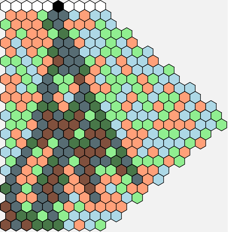
The design of a discrete neural network in this project is a grid of hexagonal grid. Each hexagon represents a “gating cell” or a “cell” which implements a certain binary operation. The hexagon shape is chosen such that the input are the top two phases of the shape are defined as the inputs. During the forward pass, the input row with certain activated (shaded) elements are fed to the next row. For each hexagon in the row, the two input faces are used as inputs for the binary operation.
Each cell can be one of the following binary operations:
Each cell can be one of the following binary operations:
1
.AND: Only true if both inputs are true.
2
.OR: True if at least one of the inputs are true.
3
.XOR: True if exactly one of the inputs are true.
These specific cell types were chosen due to their empirical superior performance compared to others during testing. Other gates tested were NONE (always false, equivalent of classical dropout) and NAND (logical inverse of AND) which severely degraded performance. Due to the training algorithm described below, the network has the ability to choose which gating types to use.
Taking inspiration from traditional neural networks that embed inputs into a higher dimensional “hidden dimension” [6], this project incorporates a “ramped” network design that allows the networks a “hidden space”. This design has several benefits that have been observed during training processes: allowing a network to “sink” activated gates [7], and allowing the network to have more flexibility in configuration.
The models in this work are exclusively scalar in, scalar out. This is due to the encoding/decoding strategy employed to convert from real to discrete and discrete to real values (encoding: RealToOneHot10, decoding: OneHot10ToReal). Inputs are converted to a one-hot vector of 10 bits and the outputs are decoded, both in accordance with the encoding/decoding functions described in the previous functions. The input one-hot vector is represented as fake “layer” at the top of the network in visualizations.
Demonstration of the forward pass
Demonstration of the forward pass
Here, the rampLength variable controls how many for how many rows the columns increases, and then decreases. To maximize the area of the “hidden” space, this is defined as half the rows.
First, define parameters that control the shape of the neural network:
rows=24;cols=10;rampLength=rows/2;
Next, we initialize the network’s weights. This will create weights randomly initialized from {AND, OR, XOR}.
weightDataRamp=CreateRampedWeights[rows,cols,rampLength];
Created 372 weights for ramped architecture
Finally, running the model is relatively easy. This gives the input scalar 0.5 and information about the network’s shape:
output=DiscreteNetRealOneHot[0.5,weightDataRamp,Visualize->True,Rows->rows,RampLength->rampLength];
The numerical output of the neural network is at index 1:
In[]:=
output[[1]]
Out[]=
1.5
Because we set Visualize->True, the returned visualization can be found at index 2:
In[]:=
output[[2]]
Out[]=
Training algorithm
Training algorithm
During training, the following genetic-style approach is used:
1
.Run several mutated variants of the current best-performing weights as a “microbatch” to determine which performs best with the given loss function.
2
.The best-performing variant in the “microbatch” is used to compare against and potentially replace the running best-performing variant.
3
.This best-performing variant is used as the model for the next training.
To measure performance, an error value is used. This is L1 loss (maximum absolute error or MAE) and is used to define the best performing model on a linear scale.
In particular, training uses several components:
a) Learning rate: a decreasing mutation rate as training progresses. Because mutation rate is analogous to the learning rate in continuous machine learning, the decreasing learning rate takes inspiration from continuous machine learning. Techniques such as learning rate scheduling in continuous machine learning change the rate that the network’s weights are updated as the model trains, improving convergence.
b) Optimizer: using simulated annealing. Discrete neural networks are not compatible with traditional continuous training techniques like backpropagation. While techniques like BOLD [4] exist, they require relaxing the continuous constraint during training. Instead, simulated annealing works by occasionally accepting worse solutions with a certain probability. Like the continuous optimizer analogy of momentum, this helps to escape settling in local minima in the optimization landscape.
c) Random restart: restart training if progress plateaus for a set amount of steps. This serves a similar purpose as the simulated annealing algorithm, but is a more coarse and unforgiving approach.
d) Penalty: due to the fact that activations in discrete neural networks are not guaranteed to reach the output, a large penalty value is applied to the error value in the case that the network does not produce an output and the expected output should have one. Essentially, if the activations did not “reach” the bottom but should have, this variant is unsuccessful regardless of performance on other inputs.
Because the encoder and decoder functions are designed to return the sum of the activated outputs (0.1+0.3, for example), the model is allowed to learn more complex and flexible representations with alternative answers. As can be seen in further experiments, this is utilized by the model to enhance flexibility.
Preparing the parallelization environment
Preparing the parallelization environment
To improve performance during the training process which tests multiple mutated weights at once, we define a parallelization factor. This sets how many candidate variants with different mutations will be tested for each training step:
numParallelVariants=64;
To fully utilize all the computer’s cores, we launch parallel kernels. If there are 8 cores, then each kernel will run 8 different mutations:
LaunchKernels[]
Finally, in order to properly implement parallelized processing, we must load the pack on each parallel kernel.
In[]:=
ParallelTable[CloudGet@"https://www.wolframcloud.com/obj/ericlbuehler/WSRP25/DiscreteNetUtil";,{numParallelVariants}];
Hyperparameter setup
Hyperparameter setup
First, we clear some variables to ensure a clean environment:
ClearAll[weightData,weightDataNew,bestPreviousError,bestWeight,y,x,target]
Here, we define some variables that will be used by the training loop. These are updated progressively as the best network is found.
bestWeight=weightData;bestError=10^10;currentError=bestError;
Next, we define training hyperparameters. These are empirically determined to work well, and control the rate of simulated annealing, mutations for each variant, random restart threshold, and maximum iterations:
maxIterations=50000;initialTemp=1.0;finalTemp=0.001;mutationRate=12;minMutationRate=1;adaptiveFactor=0.99;restartThreshold=5000;penaltyValue=10^6;
Finally, these scratch variables are used during training to track various metadata about the training run:
errorHistory={};itersSinceImprovement=0;
Weight initialization
Weight initialization
Define the model’s shape: 24 rows ramping up and down for the first 12 and last 12 respectively. There are 10 columns for the input and output as is necessary due to the encoding/decoding strategy in RealToOneHot10 and OneHot10ToReal.
rows=24;cols=10;rampLength=rows/2;
Finally, create the weights for the model:
weightData=CreateRampedWeights[rows,cols,rampLength];
Created 372 weights for ramped architecture
Defining input and target data
Defining input and target data
Define the training data x and the target values to train against. There are multiple target data, simulating f(x) as a linear function, as an trigonometric function, and as a discrete oscillatory function:
x=Table[v,{v,0,1.0,0.1}];
target={0.0,0.1,0.2,0.1,0.0,0.1,0.2,0.1,0.0,0.1,0.2};
ListPlot[Partition[Riffle[x,target],2]]
This round-trip shows the target values we would expect for each x if the model was perfectly accurate:
Training utility functions
Training utility functions
It is useful to define utility functions for training. The following ones implement core logic regarding error calculation and the simulated annealing strategy.
This function simply wraps the network evaluation function, and runs the model with the given inputs:
This function wraps the network evaluation function and contains logic for evaluating the error as well as potential penalty values. It runs the model with the given inputs, computes the error value, and applies the penalty value:
This implements simulated annealing, where there is a changing probability for worse results to be occasionally accepted and escape local minima in the training loss landscape:
Training algorithm walkthrough
Training algorithm walkthrough
Below is a walkthrough of the body of the main training loop. The entire training loop is defined as the function TrainDiscreteNet in the “Training Loop” section.
Define parameters describing the simulated annealing temperature as well as the current mutation rate. These define the probability that a worse solution would be accepted and the number of weights that will be mutated for each variant, respectively:
Next, create several mutated variants of the current best weights. A controlled number of gates are randomly updated.
Run each variant on the same inputs and find the error for each variant:
Find the best variant by the error to the target:
This implements the logic to decide whether to accept. If the error is better than the penalty value and the current best is the penalty value, then always accept. However, otherwise, use the simulated annealing strategy to decide acceptance:
Based on the acceptance condition, we can now update the current best weight and best error:
Increment the counter that tracks the number of iterations since an improvement:
In the case that the network has settled in a high-error local minima, we can execute a hard restart:
This is the entirety of the training algorithm.
How does the dataset and depth affect performance of discrete neural networks?
How does the dataset and depth affect performance of discrete neural networks?
In this section, the exploration aims to identify which kinds of functions can be effectively captured by discrete neural networks of various sizes. The objective is to understand the relationship between the complexity of the target function and the size of the discrete neural network required to model it. By systematically varying the model size - characterized by the number of discrete logical gates - we observe how accurately networks can represent different categories of functions, including linear, cyclic, and trigonometric patterns. This experiment provides insight into the minimal complexity required for reliable function approximation, potentially revealing inherent trade-offs between model size and accuracy in discrete neural networks.
Preparing the RemoteBatchSubmit environment
Preparing the RemoteBatchSubmit environment
Initialize and install the required paclets to interface with RemoteBatchSubmit.
These next few cells allow you to check if you are connected and everything is correctly set up:
Creating input data and various kinds of target data
Creating input data and various kinds of target data
Now, we create the various target functions to model: “linear” (a linearly increasing function), “trig” (a sine wave), and “osc” (an oscillatory function similar to a sawtooth wave.
Here we define 4 network configurations. This is organized as {row count, ramp length}. This defines 4 decreasing network sizes.
Launching the grid to train each case
Launching the grid to train each case
Create the grid to train for each, pairing each network configuration with one of each target data. This creates a grid of network configuration to target data.
This grid has 12 configurations: 4 network and 3 functions. We will train each configuration:
The grid looks like the following.
This function handles dispatching the batch run for each item in the grid. Like in previous sections, it is required to initialize the parallel kernels by loading the packages:
Finally, we can launch the training run over the entire grid:
While running the job, you can check the status.
Or, you can check the log for a more detailed status.
Once the job is done, we extract the results into a list.
The most important result is the final error value.
Analyzing the results
Analyzing the results
Here, we plot models with different model sizes but the same target data to compare performance of the model.
To compare the final error value with the model’s training configuration, we can pair the grid to the final error values so the inputs and outputs are connected:
Now, we can process the paired results to generate a graph to understand the best configuration of the network for each dataset!
We can delete duplicate target data patterns so that we are only grouping by meaningful data.
Next, we create labels for each of these target patterns. Each target data point has its own pattern, which can be used to find the correct label:
Group data by target pattern. In the end, models with different sizes but the same target data will be plotted in the same graph to achieve the desired comparison.
Get the 3 target patterns corresponding to the 3 target datasets:
Finally, create a visualization for each grouping of target data to model size.
The completed scatter plots reveal a clear capacity ladder.
Errors for the linear task collapse below 0.4 once the model reaches ~20 rows and flatten thereafter.
Cyclic (sawtooth) tasks tolerate roughly five fewer rows of under-fit before crossing the same threshold.
The trigonometric task falls in between: its smoothness eases approximation, yet its periodicity still needs more capacity than the linear baseline but less than the staircase.
Across all three patterns, additional width beyond ~20 rows typically yields diminishing returns, marking that band as the practical sweet-spot for subsequent experiments. The key outlier is the trigonometric task which performs better as the model size increases. This could be due to the increased task complexity.
The results clearly highlight a pattern where specific functions inherently require different minimal network sizes to achieve low error. For simpler functions, like linear patterns, smaller models perform adequately, maintaining low error rates. However, more complex functions - such as those exhibiting cyclic or trigonometric behavior - show a steep increase in error when modeled by smaller networks, indicating the necessity of larger, more complex architectures for accurate representation. This exploration underscores the importance of carefully matching model size to the type of function, affirming that discrete neural networks’ capacities strongly correlate with both structural complexity and the intrinsic characteristics of the functions they approximate.
How are the weights of discrete neural networks affected by their dataset?
How are the weights of discrete neural networks affected by their dataset?
This section investigates whether discrete neural networks, after successfully learning to represent a given function, reflect identifiable patterns within their learned weights. Specifically, we analyze discrete weights represented by logical gates (such as AND, OR, and XOR) to detect systematic structures correlated with the functions they model. By visually and computationally inspecting these weight patterns, this section seeks to uncover if specific gate distributions emerge consistently for certain types of functions. Such insight would confirm that discrete neural networks not only memorize input-output relationships but also encode meaningful structural characteristics inherent to their learned tasks. By intentionally over-fitting the model to the data, we can ensure that the weights encode as much memorization of the target dataset as possible and provide the best opportunity to expose any patterns.
Defining input and target data
Defining input and target data
First, we create our input data:
Then, we create a very simple stepped set of target values to define a very distinctive function which is easy to learn.
This forms a very simple piecewise function with a step:
Launching a training run
Launching a training run
Because the dataset is so simple, very few iterations are required to achieve zero error (complete memorization). However, memorization here is good for understanding how weights are affected by the dataset.
We can now train the discrete neural network and intentionally over-fit it. Because the network is very simple, training it for only 50 steps is sufficient to over-fit.
To make visualizing the outputs of the neural network trained in this way, pre-trained weights have been hard-coded below. To use your own, replace this cell with result = %;.
Visualizing patterns in the trained weights
Visualizing patterns in the trained weights
This interactive visualization clearly illustrates striking patterns within the trained discrete neural network. For each distinct output value (0.0 and 1.0 from the target dataset) the model exhibits a highly structured internal behavior. After an initial series of rows characterized by dynamic gate switching, the network consistently settles into a stable, fixed logical path, indicating that these early rows effectively serve as adaptive routing mechanisms directing inputs into predictable, stable computational pathways.
An intriguing example of emergent behavior occurs when representing the 1.0 output: rather than directly activating the cell labeled explicitly for “1.0,” the network cleverly combines activations from “0.2” and “0.8” cells. This pattern is a direct result of the behavior of the OneHot10ToReal function, and was never trained for. This phenomenon shows that discrete neural networks do not merely encode memorized input-output mappings; instead, they form a computational narrative, transparently revealing the internal logic and mechanisms behind the function the network implements.
An intriguing example of emergent behavior occurs when representing the 1.0 output: rather than directly activating the cell labeled explicitly for “1.0,” the network cleverly combines activations from “0.2” and “0.8” cells. This pattern is a direct result of the behavior of the OneHot10ToReal function, and was never trained for. This phenomenon shows that discrete neural networks do not merely encode memorized input-output mappings; instead, they form a computational narrative, transparently revealing the internal logic and mechanisms behind the function the network implements.
Conclusion and Next Steps
Conclusion and Next Steps
We have demonstrated that discrete neural networks exhibit distinct patterns in how their complexity and internal structure correlate with their ability to model various classes of functions. The analysis of network size versus performance across linear, cyclic, and trigonometric functions highlighted critical insights: larger networks generally improved modeling capabilities, yet the relationship varied notably across function types. Furthermore, visualizations of intentionally over-fit network weights provided clear indications that discrete neural networks encode functional characteristics distinctly within their structural parameters.
Additionally, the genetic-inspired simulated annealing training algorithm employed offers significant advantages over traditional backpropagation methods. Since discrete neural networks rely on logic gate structures (AND, OR, XOR) rather than differentiable activation functions, standard gradient-based optimization techniques like backpropagation are infeasible. The simulated annealing approach effectively navigates the non-differentiable landscape by exploring a broader range of network configurations, thus optimizing the discrete structures directly without the need for gradient information.
Moving forward, several promising directions warrant further exploration:
1
.Expanded Function Set Analysis: Investigating additional function categories, such as exponential, logarithmic, or piecewise-defined functions, will clarify the broader applicability of discrete neural networks.
2
.Deeper Structural Analysis: Performing more detailed and systematic weight pattern analyses using quantitative metrics and advanced visualization techniques can help better understand the intrinsic encoding mechanisms of discrete neural networks.
3
.Optimization and Generalization: Evaluating methods that enhance generalization, such as modified genetic algorithms or hybrid training approaches, will further refine the practical applicability of discrete neural networks in modeling complex functions.
These next steps will build upon the findings presented here, guiding future research toward a deeper theoretical understanding and improved practical implementations of discrete neural network models. However, due to scaling challenges, it may be difficult to effectively grow these networks to the required sizes for practical applications. The primary limitation of networks described in this work are scalar in, scalar out. Another key limitation is the accuracy used to encode one number: encoding and decoding accuracy suffers due to the large step size of 0.1 in the encoding/decoding functions.
Regardless, solving these limitations could enable discrete neural networks as a viable alternative to continuous strategies in certain applications of machine learning such as edge environments.
Regardless, solving these limitations could enable discrete neural networks as a viable alternative to continuous strategies in certain applications of machine learning such as edge environments.
Acknowledgements
Acknowledgements
I’d like to thank my wonderful mentor, Anton Antonov, for his support and guidance throughout my project. I would also like to thank the directors Rory Foulger, Eryn Gillam, and Megan Davis for providing compute resources that I used to complete this project. Finally, I want to thank Dr. Stephen Wolfram for introducing me to topic of discrete neural networks.
References
References
1
.Wolfram, S. (2024, August 22). What’s really going on in machine learning? Some minimal models. Stephen Wolfram Writings. Retrieved July 9, 2025, from https://writings.stephenwolfram.com/2024/08/whats-really-going-on-in-machine-learning-some-minimal-models/
2
.Engel, J. (1988). Teaching feed-forward neural networks by simulated annealing. Complex Systems, 2, 641–648. https://wpmedia.wolfram.com/sites/13/2018/02/02-6-2.pdfs
3
.Bernal, J., & Torres-Jimenez, J. (2025). SAGRAD: A program for neural network training with simulated annealing and the conjugate gradient method. arXiv preprint arXiv:2502.00112. https://arxiv.org/abs/2502.00112
4
.Nguyen, V. M. (2024, May 7). Boolean variation and Boolean logic backpropagation (arXiv:2311.07427v2) [Preprint]. arXiv. https://doi.org/10.48550/arXiv.2311.07427
5
.Courbariaux, M., Hubara, I., Soudry, D., El-Yaniv, R., & Bengio, Y. (2016). Binarized neural networks: Training deep neural networks with weights and activations constrained to ±1. https://arxiv.org/abs/1602.02830
6
.Rumelhart, D. E., Hinton, G. E., & Williams, R. J. (1986). Learning representations by back-propagating errors. Nature, 323(6088), 533–536. https://doi.org/10.1038/323533a0
7
.Zhang, S., Khan, M., & Papyan, V. (2025, February 2). Attention sinks and outlier features: A “catch, tag, and release” mechanism for embeddings (Version 1) [Preprint]. arXiv. https://arxiv.org/abs/2502.00919
CITE THIS NOTEBOOK
CITE THIS NOTEBOOK
Training and exploring the inner workings of discrete neural networks
by Eric Buehler
Wolfram Community, STAFF PICKS, July 10, 2025
https://community.wolfram.com/groups/-/m/t/3499426
by Eric Buehler
Wolfram Community, STAFF PICKS, July 10, 2025
https://community.wolfram.com/groups/-/m/t/3499426