ORIGINAL ARTICLE: Housam Binous, Equilibrium Staged Separations using Matlab and Mathematica, Chemical Engineering Education, Vol. 42 No. 2 (Spring 2008) pp. 69-73. DOI: https://journals.flvc.org/cee/article/view/122382
Article Abstract: We show a new approach, based on the utilization of Matlab and Mathematica, for solving liquid-liquid extraction and binary distillation problems. In addition, the author shares his experience using these two softwares to teach equilibrium staged separations at the National Institute of Applied Sciences and Technology.
Some binary mixtures, such as water and ethanol, have a non-ideal behavior that is characterized by the presence of a positive azeotrope. This minimum-boiling azeotrope makes the preparation of anhydrous ethanol a challenging task that requires special techniques, such as extractive distillation and heteroazeotropic distillation using ethyleneglycol and benzene as entrainers, respectively.
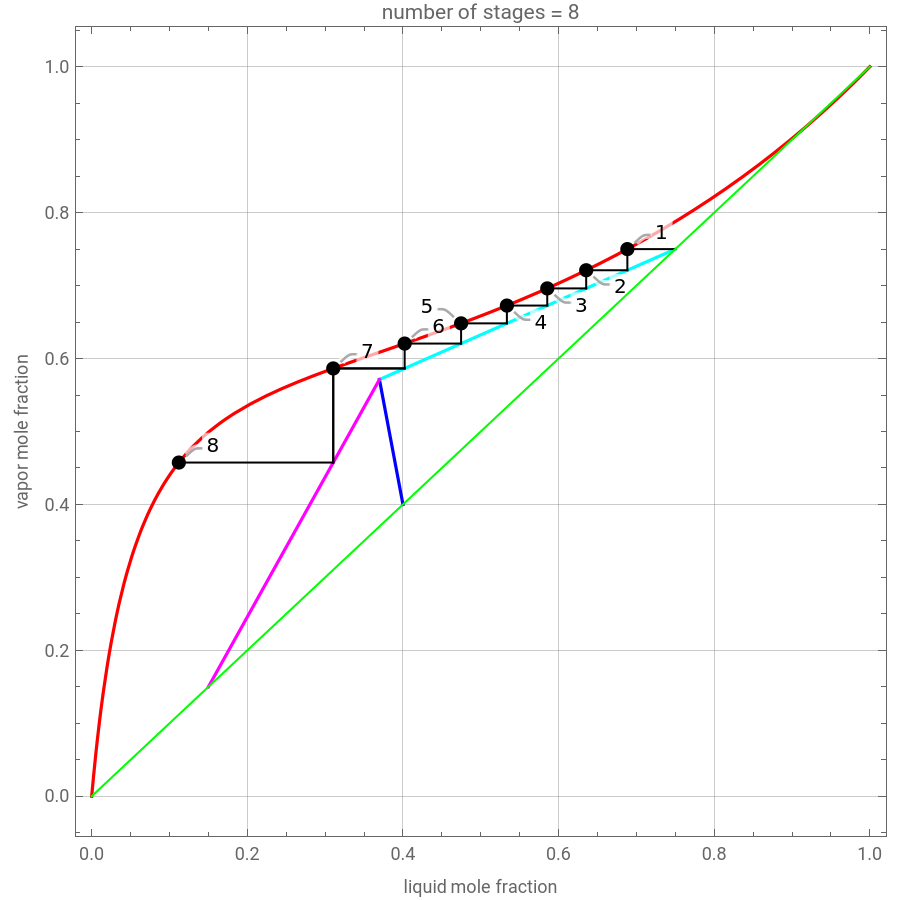
Here, we present the McCabe-Thiele graphical method applied to the water-ethanol mixture. First, the rectifying (cyan) and stripping (magenta) operating lines are plotted using a reflux ratio equal to 1.5 times the minimum reflux ratio. These lines are derived by writing global and partial material balances around different sections of the column. The feed line (black) is also plotted. If the construction is correct, these three lines must intersect at the same point. For the separation to be feasible, you must choose values for the parameters' feed quality, bottom, feed and distillate compositions that cause the intersection point to fall below the equilibrium curve (red).
The equilibrium curve is obtained using the van Laar model for the computation of the activity coefficients, which are used in the modified Raoult’s law. The stages are stepped off using the equilibrium curve and the two operating lines in order to determine the number of equilibrium stages or the number of theoretical column plates. The points that allow the construction of the steps are alternatively on the equilibrium curve or on the operating line. If one point is on the equilibrium curve, it corresponds to two streams in equilibrium leaving a particular stage. When the point is on the operating line, it corresponds to two passing streams, one entering and one leaving the stage. The horizontal and vertical axes are the liquid and vapor mole fractions. The red curve is the equilibrium curve. In fact, every liquid with mole fraction is in equilibrium with its vapor with mole fraction . The line segments allow a visualization of the steps, which are equilibrium stages.
x
y
One limitation of this approach is that it will not work when the feed is saturated vapor (feed quality ), because the slope of the feed line becomes infinite. We display the number of stages, which is the sum of the plates in the rectifying and stripping sections. The optimum feed plate is the stage where the operating lines intersect. If the user sets the distillate specification close to the azeotropic composition, then the number of plates becomes very large. Indeed, there is a severe tangent pinch (i.e., the operating line is almost tangent to the equilibrium curve).
q=1
Feed, distillate and bottom specifications .
In[]:=
xd=0.75;xb=0.15;zf=0.4;q=0.85;
VLE data based on Modified Raoult’s law, van Laar activity coefficient model and Antoine equation
A2=8.07131;B2=1730.630;C2=233.426;A1=8.11220;B1=1592.864;C1=226.184;PS1=10^(A1-B1/(C1+T));PS2=10^(A2-B2/(C2+T));G1[i_]:=Exp[A12(A21(1-x[i])/(A12x[i]+A21(1-x[i])))^2];G2[i_]:=Exp[A21(A12x[i]/(A12x[i]+A21(1-x[i])))^2];A12=1.6798;A21=0.9227;i=0;P=760;While[i<101,{x[i]=i0.01,T[i]=FindRoot[PPS1G1[i]x[i]+PS2G2[i](1-x[i]),{T,80},AccuracyGoal5][[1,2]],y[i]=PS1G1[i]x[i]/P/.TT[i],i++}];tb=Table[{x[i],y[i]},{i,0,100}];equilb=Interpolation[tb];
Feed line
feed[x_]:=If[q≠1,(qx/(q-1)-zf/(q-1))];
plt0=Plot[equilb[x],{x,0,1},PlotStyleRGBColor[1,0,0],FrameLabel{"liquid mole fraction","vapor mole fraction"},FrameTrue,AxesOrigin{0,0},Epilog{RGBColor[0,1,0],Line[{{0,0},{1,1}}]}];pinch=Quiet[FindRoot[feed[x]equilb[x],{x,0.5}]];xpinch=pinch[[1,2]];ypinch=feed[xpinch];
rectifying and stripping operating lines at R=Rmin
opertRect[x_]:=ypinch+(x-xpinch)/(xd-xpinch)(xd-ypinch);opertStrp[x_]:=ypinch+(x-xpinch)/(xb-xpinch)(xb-ypinch);
Reflux ratio and minimum reflux ratio
Rmin=(xd-ypinch)/(xd-xpinch)/(1-(xd-ypinch)/(xd-xpinch));R=1.5Rmin;
rectifying and stripping operating lines at R=1.5*Rmin
OpRect[x_]:=R/(R+1)x+xd/(R+1);inters=FindRoot[feed[x]OpRect[x],{x,0.7}];xinters=inters[[1,2]];yinters=OpRect[xinters];OpStrp[x_]:=yinters+(x-xinters)/(xb-xinters)(xb-yinters);
Plotting feed, rectifying and stripping operating lines
plt4=Plot[OpRect[x],{x,xinters,xd},PlotStyleRGBColor[0,1,1]];plt5=Plot[OpStrp[x],{x,xb,xinters},PlotStyleRGBColor[1,0,1]];plt6=Plot[feed[x],{x,xinters,zf},PlotStyleRGBColor[0,0,1],PlotRange{{0,1},{0,1}}];
stepping off stages
yr[0]=xd;xr[0]=xd;i=0;While[xr[i]>xinters,{v=Quiet[FindRoot[yr[i]equilb[u],{u,0.7}]][[1,2]],t=OpRect[v],If[v>xinters,{xr[i+1]=v,yr[i+1]=t}],i++}];ir=i-1;i=0;If[ir≥0,ys[0]=yr[ir];xs[0]=xr[ir]];While[xs[i]>xb,{v=Quiet[FindRoot[ys[i]equilb[u],{u,0.5}]][[1,2]],t=OpStrp[v],xs[i+1]=v,ys[i+1]=t,i++}];imax=i-1;
building staircase construction
If[ir≤0||imax≤0,Graphics[Text["Unfeasible distillation parameters should be changed",{0,0}],ImageSize{500,300}],tbl1=Table[Line[{{xr[i],yr[i-1]},{xr[i],yr[i]}}],{i,1,ir}];tbl2=If[ir≥1,Table[Line[{{xr[i],yr[i]},{xr[i+1],yr[i]}}],{i,0,ir-1}],Table[Line[{{xr[i],yr[i]},{xr[i+1],yr[i]}}],{i,0,0}]];tbl3=Table[Line[{{xs[i+1],ys[i]},{xs[i+1],ys[i+1]}}],{i,0,imax-1}];tbl4=Table[Line[{{xs[i-1],ys[i-1]},{xs[i],ys[i-1]}}],{i,1,imax+1}];tblih=Line[{{xs[1],ys[0]},{xr[ir],ys[0]}}];tbliv=Line[{{xs[1],ys[0]},{xs[1],ys[1]}}];it=imax+ir+1;]
McCabe & Thiele graphical construction construction.
We display the total number of stages (8 stages). Optimal feed stage location is 7th stage (counting from the top).
We display the total number of stages (8 stages). Optimal feed stage location is 7th stage (counting from the top).
In[]:=
Show[plt0,plt6,plt4,plt5,ListPlot[Join[Table[{xr[i],equilb[xr[i]]},{i,1,ir}],Table[{xs[i],equilb[xs[i]]},{i,1,imax+1}]]->Range[imax+ir+1],PlotStyle->{Black,PointSize[0.0175]}],Graphics[{tbl1,tbl2,tbl3,tbl4,tblih,tbliv}],PlotLabelStyle[Row[{"number of stages = "<>ToString[it]<>""}]],ImageSize{450,450},GridLines->Automatic,AspectRatio->1]
Out[]=
CITE THIS NOTEBOOK
CITE THIS NOTEBOOK
McCabe-Thiele Graphical Method for a Non-Ideal Binary Mixture
by Housam Binous and Ahmed Bellagi
Wolfram Community, STAFF PICKS, February 5, 2024
https://community.wolfram.com/groups/-/m/t/3116111
by Housam Binous and Ahmed Bellagi
Wolfram Community, STAFF PICKS, February 5, 2024
https://community.wolfram.com/groups/-/m/t/3116111