In this project, I implemented measures of compactness for electoral districts to find fair divisions and detect gerrymandering, or corrupt redrawing of districts. The main strategy used was generating many random districts made from counties and analyzing the fairness of each one based on simulated election results, population distribution, and several calculated compactness measures. I also applied the compactness tests to existing districts to find gerrymandering.
Introduction
Introduction
About Gerrymandering
About Gerrymandering
Gerrymandering is the process of intentionally designing electoral districts to skew the results of elections. The term was coined in 1812 by the Boston Gazette referring to the new electoral districts in Massachusetts under Governor Elbridge Gerry, as they thought one district looked like a mythological salamander.
The original Gerrymander:
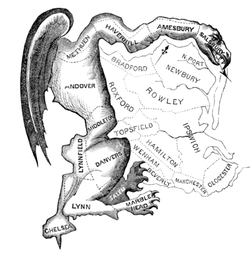
Gerrymandering can include spreading a population of one group into multiple districts where they have the minority or packing them into one district so they only win that one. The reason this has such a large impact is that votes can be wasted, either by having a slight minority or an extreme majority, and this effect can change the outcomes of elections. Therefore, the way the districts are designed is very important. There are some simple rules for creating districts:
1
.Each district must be continuous.
2
.Each district should have a similar (ideally equal) population (currently around 760,000 people).
3
.Each district should be “compact.”
Because it is difficult to judge if a district is compact or not, many methods have been created to quantify how gerrymandered districts are. In this project, I quantified these characteristics and determined both which current districts are the most gerrymandered and create some new, potentially fairer redistrictings.
Redistricting
Redistricting
A common strategy in finding fair electoral districts is generating large numbers of random districts and determining which are the fairest. I chose to generate districts out of counties, both because it preserves existing boundaries and because counties are essentially the smallest division the Wolfram Knowledgebase supports.
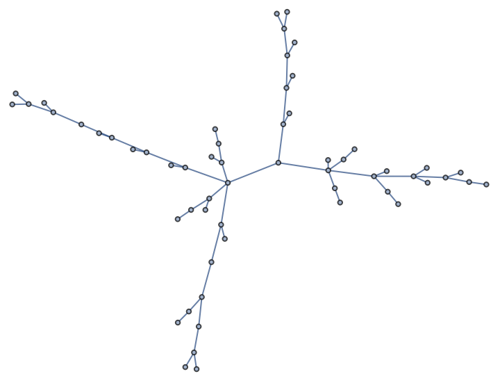
An easy way to generate districts while ensuring that they are all continuous is by creating a spanning tree of a graph of the counties, where only adjacent counties are connected, then cutting edges. Cutting an edge preserves adjacencies while always producing a new district.
An easy way to generate districts while ensuring that they are all continuous is by creating a spanning tree of a graph of the counties, where only adjacent counties are connected, then cutting edges. Cutting an edge preserves adjacencies while always producing a new district.
Function to make an adjacency graph of a list of counties:
In[]:=
treeify[counties_List]:=FindSpanningTree[Graph[Flatten[ Table[If[MemberQ[counties, n],xn, Nothing], {x, counties}, {n, EntityValue[x, "BorderingCounties"]}]]]]
Make a graph of California:
In[]:=
californiaTree=treeifyEntityList

Out[]=
Function to randomly split a tree into two trees by cutting a single edge:
In[]:=
splitGraph[graph_Graph]:=Graph[ VertexList[graph], ReplaceAll[EdgeList[graph], RandomChoice[EdgeList[graph]]->Nothing]]
In[]:=
splitGraph[californiaTree]
Out[]=
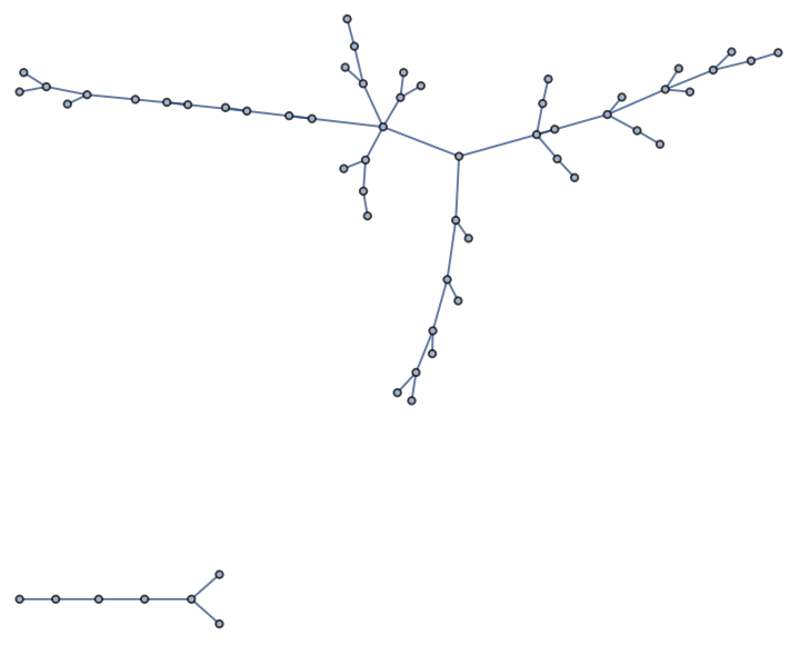
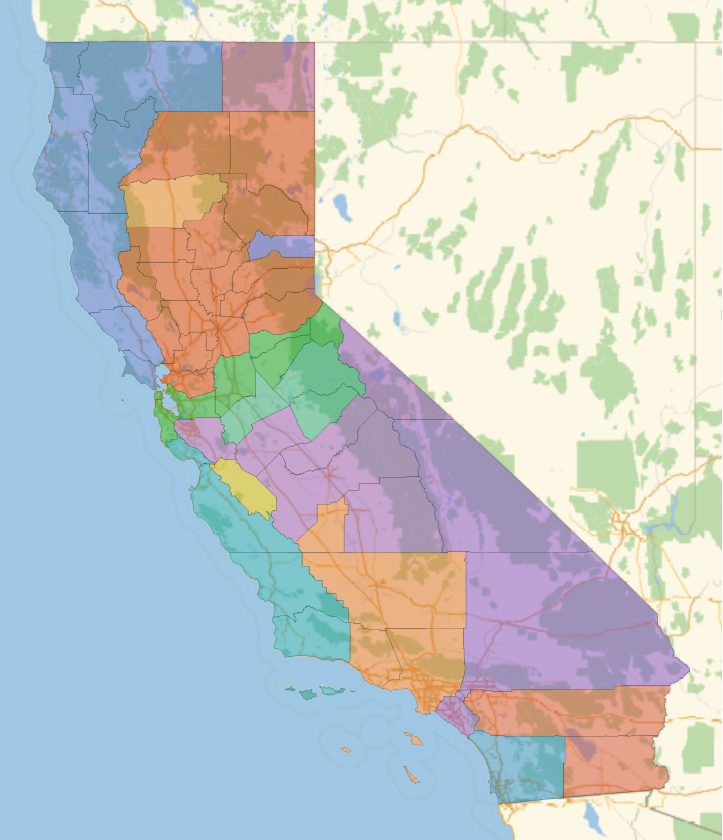
By nesting splitGraph, this function can randomly divide the whole state into some number of districts. We can use ConnectedComponents to find the new districts after using splitGraph.
Randomly divide the graph into a specified number of districts:
In[]:=
randomDistricts[graph_, num_Integer]:=ConnectedComponents[Nest[splitGraph, graph, num-1]]
In[]:=
GeoListPlot[randomDistricts[californiaTree,15]]
However, there are a limited number of possible divisions this method can produce, as it can only make districts based on the initial spanning tree. To work around these limitations, we can pick two adjacent districts in an already divided map and randomly redivide them, then repeat. This method can reach any division and can be iterated on a previous division.
Returns true if the districts border each other, false if not
In[]:=
districtsBorderQ[district1_, district2_]:=IntersectingQ[Complement[Union[Flatten[Table[EntityValue[n, "BorderingCounties"], {n, district1}]]],district1], district2]
Randomly divides two adjacent districts
In[]:=
changeTwo[districts_List]:=Module[{a =RandomChoice[districts],b, c},b=RandomChoice[Select[districts, districtsBorderQ[a, #]&]];c={a,b};Join[ConnectedComponents[splitGraph[treeify[Flatten[c]]]], Cases[Cases[districts, Except[a]], Except[b]]]]
Use Nest to repeatedly apply
In[]:=
random=Nest[changeTwo,randomDistricts[californiaTree,14],20];
In[]:=
GeoListPlot[random]
Out[]=


Voting Data
Voting Data
The result of the election is the most important factor in determining if the redistricting is fair, so we have to simulate the result with any given division.
Voting data for some of the states by county (California, Texas, Ohio, Oregon, Washington)
Function to reformat a list of voting data for a specific state into an association (input needs to be in a specific format)
Now we can find the winners given a list of districts made from counties.
Function to get the ratio of Democrat to Republican representatives for a districting:
We also need a point of reference for our new districts, so this function determines the actual ratio of voters, which ideally the ratio of district winners would reflect.
Function for ratio of Democrat votes to Republican votes based on the data
Compactness measures
Compactness measures
The other way to determine fairness is to study the shape of the districts to determine how compact they are. There are many definitions and measures, so I implemented multiple methods. First, here is a function that combines polygons of counties into a single polygon with only the outer border for analysis of the shape. There are some counties or districts that particular region functions don't work on due to holes, islands, or unknown factors, so these all have to be checked for.
Turns a list of counties into one polygon
1. Roundness
1. Roundness
The first measure of compactness is determining the "roundness" of districts (Coefficient of variation, or SD divided by mean, of the distance of each point on the boundary from the average radius):
Roundness function, takes in a district shape and outputs the coefficient of variation
An example of a round district and a long, thin district:
The top district is closer to being a circle:
The scores go up from 0, with 0 being a perfect circle. The skinnier district has a higher score, which means it is less round.
2. Polsby-Popper Test
2. Polsby-Popper Test
A standard method to quantify the compactness of a district is to calculate 4π multiplied by the ratio of the area to the perimeter squared, which is known as the Polsby-Popper Test. This number has no units, so the size of the district doesn't matter. The scores range from 0 to 1, where 1 is better. Inputting a perfect circle would return 1.
Function that takes a polygon and returns the value of the Polsby-Popper test
Again, the rounder district gets a better score.
3. Reock Test
3. Reock Test
The Reock Score measures a similar quality. It is the ratio of the area of the district to the area of the smallest bounding circle (1). It punishes long offshoots heavily.
Reock Test function, takes in the shape of a district and outputs a number between 0 and 1, with 1 being ideal.
Sierra Leone is very round and gets a high score, while Chile is long and thin and gets a low score
4. Population
4. Population
Ideally, the population of each district would be exactly the same. This function determines how evenly distributed the population of the state is between districts. The scores start from 0, where a lower score is better.
Return the coefficient of variation for the populations of the districts:
Some populations in "random" (California example from above) are very high and others are very low, so the output of the function is high.
These counties have very similar populations, so the output is low.
This is a function to determine how spread out the population is within each district. This matters because one gerrymandering technique is connecting cities with thin strips of land to weaken their voting power, so the test punishes having large populations on the edges of the district. It is calculated by the average distance of each person from the centroid divided by the average radius, where each county counts as a population at its centroid.
Returns (population of each county * distance from its center to the center of the district)/(total population of the district * average radius of the district), which has no units:
The long district with the majority of the population (Los Angeles) on one end gets a high output, and the compact district gets a lower output.
A more accurate evaluation could be made by implementing cities as the population centers instead of only whole counties, but this is difficult. One major problem of using counties as the smallest unit is having very large counties like Los Angeles County that have millions of people but can’t be split up into multiple districts.
5. X-Symmetry
5. X-Symmetry
The final test is X-Symmetry. To calculate it, we rotate the shape by π radians and find the ratio of the area of the overlap with the original image to the area of the original image using DominantColors. See below for examples. The score ranges from 0 to 1, with 1 being better.
(Traditionally, the district is reflected over the x-axis (1), but it is easier to rotate the polygons and the result is approximately the same).
(Traditionally, the district is reflected over the x-axis (1), but it is easier to rotate the polygons and the result is approximately the same).
Returns ratio of overlap area to original area
The thin, asymmetrical district gets a lower, worse score than the compact one.
Applications
Applications
Analyzing random districts made from counties
Analyzing random districts made from counties
Now, we want to find the fairest way to redraw districts for any given area. The steps to do this are:
1
.Generate random districts.
2
.Use changeTwo to continuously make new districts.
3
.Determine fairness by election results and compactness for each redistricting.
4
.Find the district with the best score.
To implement this, here is a function to combine all of the compactness measures that look at individual districts, then a function to analyze an entire state.
Returns a compactness score for a district. Not evenly weighted because the ranges for some functions are different.
Fairness of the districting of an entire state. Somewhat arbitrary coefficients, would need fine-tuning. Currently ranges from 12 (uniform, perfect circles) to negatives.
Now, we iterate over a sample size of our choosing:
Returns the “fairest” redistricting out of a chosen number randomly generated ones for a state based on compactness scores and the given voting data.
We can repeat the process with a better districting as input, as a Markov chain Monte Carlo:
Start from a previous good districting and continue from there instead of a random start
This will produce good results, though it is computationally intensive and can get stuck in local maxima if the number of divisions generated is not large enough.
Some examples
Some examples
Applying the function to some actual states:
Oregon
Oregon
Get the voting data:
Find the fairest distribution out of 10. To get my results, I used sample sizes of a few thousand.
This division was relatively fair, and it can be seen that the larger districts are in areas with smaller populations, but are still "compact."
Washington
Washington
Repeat the same for other states:
This division looks stranger due to the one large district, but it is averaged out by the voting fairness and relatively even population distribution.
California
California
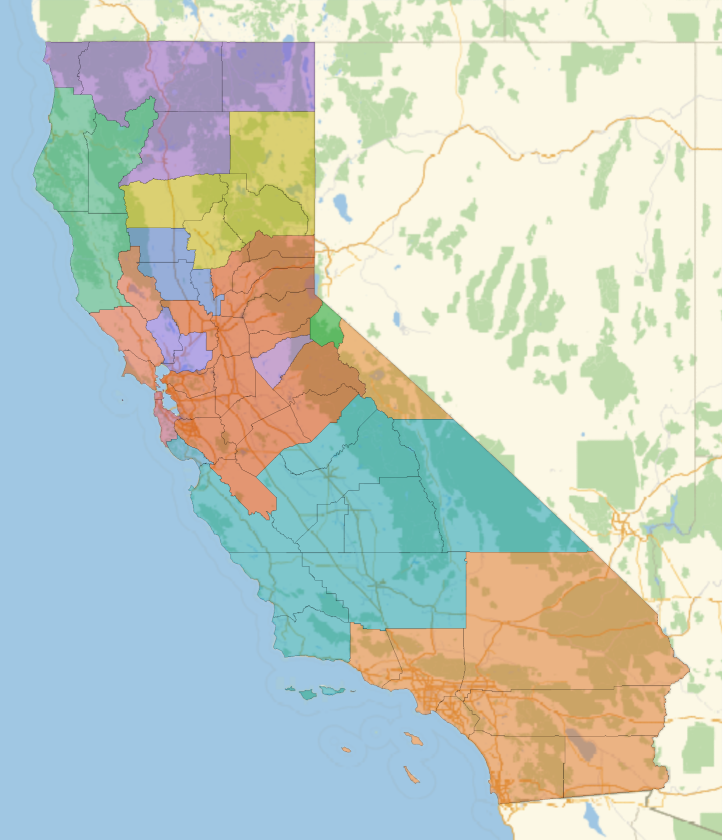
California has a very high population but proportionately few counties, so I needed to decrease the number of districts to create variety.
A good population distribution is difficult to achieve with only counties here.
Actual Districts
Actual Districts
I also wanted to apply my compactness measures to actual congressional districts. Here are the functions adapted for district objects instead of lists of counties:
Get the largest polygon in the district:
Find the perimeter:
Polsby-Popper:
Roundness:
Reock:
X-Symmetry
Total compactness score for the district:
Now, we can look at all of the districts in the US at the same time and find the best and worst ones:
Get the districts and their polygons (Remove those without data and those that are entire states (2)):
Get the compactness score for each district:
Find the worst few districts:
And the best 5:
Sure enough, the worst districts are long and spindly, while the best are mostly very round. The best district (Hawaii second congressional district) is missing the rest of the islands because I only took the largest polygon in each district.
Conclusion
Conclusion
This project was effective in implementing techniques for determining compactness and produced some good results. Finding good compactness measures is a point of contention in modern politics, and there are many disagreeing viewpoints. Studies like this one can be very effective in preventing gerrymandering and detecting it when it occurs. This is an important issue, and quantifying fairness can and will change the course of elections.
There are still some issues, like the long runtime and limited detail of counties.
◼
I could fine-tune the coefficients of the scores so that they are weighted better. There are some qualities that are not punished or rewarded as much as they should be.
◼
For example, Maryland's third congressional district was rated only seventh worst, even though it looks extremely gerrymandered, while others rated lower than it are less obviously egregious.
◼
With more computing power and/or time, I could look at a larger sample of randomly generated districts to make more fair divisions, as well as other states.
◼
I could also implement other measures of fairness, like the efficiency gap, or look at other factors, like ethnic groups, preserving previous borders, or looking at natural boundaries that might cause irregular shapes.
◼
For more precision, I could look at cities instead of only counties, and potentially divide up counties with large populations. In real life, large cities contain multiple districts, and this is not possible only using counties.
Acknowledgements
Acknowledgements
I would like to thank my mentor, Anika Patel, for helping me stay on track and improve my work. I am also thankful for Stephen Wolfram and everybody else at the Wolfram High School Summer Research Program for ideas and assistance.
Sources
Sources
1. Fisher, Z. (2016). Team 609. https://fisherzachary.github.io/
2. Pisanty, E. (2016, July 3). How can I use Mathematica to sort the US congressional districts by perimeter/area. Mathematica Stack Exchange. https://mathematica.stackexchange.com/questions/119944/how-can-i-use-mathematica-to-sort-the-us-congressional-districts-by-perimeter % C3 % B7ar
2. Pisanty, E. (2016, July 3). How can I use Mathematica to sort the US congressional districts by perimeter/area. Mathematica Stack Exchange. https://mathematica.stackexchange.com/questions/119944/how-can-i-use-mathematica-to-sort-the-us-congressional-districts-by-perimeter % C3 % B7ar
CITE THIS NOTEBOOK
CITE THIS NOTEBOOK
Create geographic compactness measurements for randomly generated districts
by Isaac McGreevy
Wolfram Community, STAFF PICKS, July 13, 2023
https://community.wolfram.com/groups/-/m/t/2962700
by Isaac McGreevy
Wolfram Community, STAFF PICKS, July 13, 2023
https://community.wolfram.com/groups/-/m/t/2962700