Description
This notebook simulates the elution of a binary mixture through a packed chromatographic column. Band propagation is described by the equilibrium-dispersive (ED) model: the two solutes are carried along by convection, broadened by an apparent axial dispersion coefficient that lumps together all band-broadening effects, and are assumed to be in adsorption equilibrium with the stationary phase at every point of the column.
The solutes are assumed to follow a linear (Henry) adsorption isotherm, so they do not compete for adsorption sites and the two partial differential equations are uncoupled. The system is solved numerically with NDSolve (method of lines), and the outlet chromatograms are compared with an analytical Gaussian approximation based on the retention time, the Péclet number and the width of the injection pulse.
Governing equations
Mass balance of solute in the column ():
i
i=1,2
∂
c
i
∂t
∂
q
i
∂t
∂
c
i
∂z
D
a
2
∂
c
i
∂
2
z
with the phase ratio
F=
1-ϵ
ϵ
and the linear (Henry) isotherm, in which each solute adsorbs independently of the other:
q
i
a
i
c
i
The time derivative of is
q
i
∂
q
i
∂t
a
i
∂
c
i
∂t
Substituting into the mass balance gives an independent linear advection-dispersion equation for each solute:
(1+F)+u=
a
i
∂
c
i
∂t
∂
c
i
∂z
D
a
2
∂
c
i
∂
2
z
Initial and boundary conditions
Initial condition (column nearly clean; the narrow Gaussian keeps the initial and inlet conditions consistent at the corner ):
t=0,z=0
c
i
c
0,i
-10000
2
z
e
Inlet (rectangular pulse of duration ):
t
inj
c
i
c
0,i
t
inj
c
i
t
inj
Outlet (no diffusive flux at the column end):
∂
c
i
∂z
z=L
Parameters and symbols
◼
L
u
D
a
◼
ϵ
F
◼
c
i
i
q
i
c
i
◼
a
i
◼
c
0,i
t
inj
t
end
◼
Values used: = 25 cm; = 0.1 cm/s; = cm^2/s; = 0.4 ( = 1.5); = 1, = 1.5; = 5, = 2.5; = 20 s; = 1000 s
L
u
D
a
2×
-3
10
ϵ
F
a
1
a
2
c
0,1
c
0,2
t
inj
t
end
Analytical Gaussian approximation
For a linear isotherm and a large Péclet number, each outlet peak is close to a Gaussian, which provides an analytical reference for the NDSolve result. The retention factor and the retention time of an impulse injection of solute are:
i
k
i
a
i
t
R,i
L
u
k
i
The Péclet number is the same for both solutes, and the standard deviation of the impulse response (in time) is:
Pe=
uL
D
a
σ
0,i
t
R,i
2
Pe
A rectangular injection of duration shifts the centre of the peak by and adds to its variance:
t
inj
t
inj
2
2
t
inj
12
μ
i
t
R,i
t
inj
2
2
σ
i
2
σ
0,i
2
t
inj
12
The moment-matched Gaussian, whose area equals the injected amount , is then:
c
0,i
t
inj
c
i
c
0,i
t
inj
σ
i
2π
-
2
(t-)
μ
i
2
2
σ
i
e
With the values used, Pe = 1250 and the impulse retention times are 625 s and 812.5 s. The Gaussian peaks are therefore centred at 635 s and 822.5 s, with standard deviations of about 25.7 s and 33.0 s. The approximation neglects the small residual asymmetry of the true peaks.
Workflow
1
.Define the parameters and the injection pulse.
2
.Define the linear isotherm and write the PDE system (one independent equation per solute).
3
.Set the initial and boundary conditions and solve with NDSolve.
4
.Plot the outlet chromatograms (t,L) obtained with NDSolve.
c
i
5
.Compute the analytical Gaussian approximation (retention time, Péclet number and peak width) and plot it.
6
.Overlay the NDSolve chromatograms (dashed lines) and the Gaussian approximation (solid lines).
◼
Units: lengths in cm, time in s, concentrations in consistent arbitrary units.
In[]:=
(*Two-ComponentEquilibrium-DispersiveChromatographylinearisotherm,rectangularpulseinjection*)(*Parameters(cm,s)*)L=25;u=0.1;Da=2*^-3;(*columnlength,interstitialvelocity,apparentaxialdispersioncoefficient*)eps=0.4;F=(1-eps)/eps;(*totalporosity,phaseratioF=(1-eps)/eps*)nc=2;(*numberofcomponents*)aL={1.0,1.5};(*Henryconstantsa_i*)c0=5{1,0.5};(*injected(feed)concentrationsc0_i={5,2.5}*)tinj=20;(*injectiontime*)tend=1000;(*endtimeofthesimulation;impulset_R,i=(L/u)(1+Fa_i)=625,812.5s*)
In[]:=
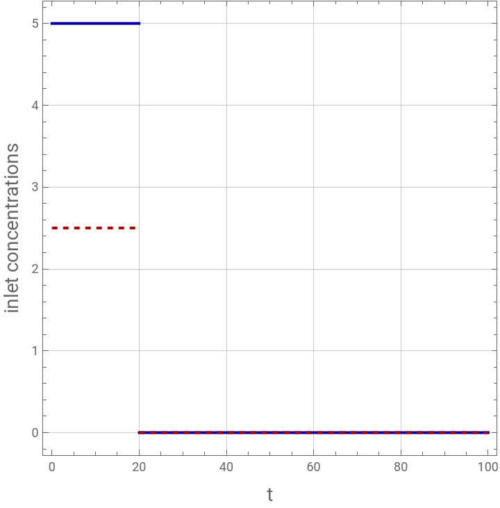
(*Injectionpulse(sameforbothcomponents)*)cin[i_,t_]:=If[t>tinj,0,If[i==1,c0[[1]],c0[[2]]]];
In[]:=
Plot[{cin[1,t],cin[2,t]},{t,0,100},Frame->True,GridLines->Automatic,AspectRatio->1,FrameLabel->{Style["t",14],Style["inlet concentrations",14]},PlotStyle->{{Darker@Blue},{Darker@Red,Dashed}},PlotLegends->{"c1 inlet","c2 inlet"}]
Out[]=


In[]:=
c={c1[t,z],c2[t,z]};
In[]:=
(*Linear(Henry)isothermq_i=a_ic_i*)q[cc_List]:=aLcc;
In[]:=
q[c]
Out[]=
{1.c1[t,z],1.5c2[t,z]}
In[]:=
(*GoverningPDEsystem*)
In[]:=
pde={(FD[q[c][[1]],t])+D[c1[t,z],t]+uD[c1[t,z],z]==DaD[c1[t,z],{z,2}],(FD[q[c][[2]],t])+D[c2[t,z],t]+uD[c2[t,z],z]==DaD[c2[t,z],{z,2}]}
Out[]=
0.1[t,z]+2.5[t,z][t,z],0.1[t,z]+3.25[t,z][t,z]
(0,1)
c1
(1,0)
c1
1
500
(0,2)
c1
(0,1)
c2
(1,0)
c2
1
500
(0,2)
c2
In[]:=
(*Initialandboundaryconditions*)ics=Table[(c[[i]]/.t->0)==c0[[i]]Exp[-10000z^2],{i,nc}];(*nearlycleancolumn;narrowGaussianmatchestheinletvalueatz=0*)bcIn=Table[(c[[i]]/.z->0)==If[i==1,If[t>tinj,0,c0[[1]]],If[t>tinj,0,c0[[2]]]],{i,nc}];(*inlet:rectangularpulseofdurationtinj*)bcOut=Table[(D[c[[i]],{z,1}]/.z->L)==0,{i,nc}];(*outlet:zeroconcentrationgradientatz=L*)
In[]:=
ics
Out[]=
c1[0,z]5,c2[0,z]2.5
-10000
2
z
-10000
2
z
In[]:=
bcIn
Out[]=
{c1[t,0]If[t>20,0,c0〚1〛],c2[t,0]If[t>20,0,c0〚2〛]}
In[]:=
bcOut