The Wolfram Language has excellent support for probabilistic modelling. However, I have long been missing support for Bayesian Networks. I got tired of relying on commercial BN tools and libraries in other languages, so I decided it was time to make my own Wolfram BN paclet. Here is a short explanation of what I did and how it works.
Introduction
Introduction
Bayesian Networks (BNs) are graphical probabilistic models for compact representation of categorical multivariate distributions . While the number of state combinations rapidly explodes with the number of variables, BN take advantage of the conditional dependencies to express distributions more efficiently in the factored form of a directed acyclic graph (DAG). For example, we could express P(X,Y,Z) as P(X)P(Y)P(Z|X,Y) if we know how Z depends on X and Y.
BNs are commonly for risk analysis and decision - support systems where one is interested in the effect of evidence on predictions.
BNs are commonly for risk analysis and decision - support systems where one is interested in the effect of evidence on predictions.
If I were to implement a BN framework in any other language, a large part of the job would probably be to implement the inference algorithms . However, the WL already has a lot of high - level functionality for probabilistic analysis . In fact, one should in principle be able to just do something like Probability[x == "A" y == "B" && z == "C", {x, y, z} dist. Moreover, the WL has a CategoricalDistribution and support for creating compound distributions using ProbabilityDistribution . However, there are two issues:
1
.It is inconvenient to use constructs like {x, y, z} dist because one has to remember the ordering of the variables.
2
.It appears that ProbabilityDistribution does not support categorical domains directly, so I had to find a workaround.
Solving issue 1 : Making Probability work with named variables
Solving issue 1 : Making Probability work with named variables
The Probability function in the WL works with multivariate distributions, however one has to specify the order of the variables, e.g., {x, y, z} dist.
To overcome this, my BayesianNetwork makes use of named variables using #name (Slot[“name”]). I then overloaded the Probability function so that it works with constructs like Probability[#var2 #var1 && #var3 &, BN].
To overcome this, my BayesianNetwork makes use of named variables using #name (Slot[“name”]). I then overloaded the Probability function so that it works with constructs like Probability[#var2 #var1 && #var3 &, BN].
Solving issue 2: Making ProbabilityDistribution work with categorical variables
Solving issue 2: Making ProbabilityDistribution work with categorical variables
To solve the second issue, I noted that there are two ways to implement categorical distributions in the WL:
In[]:=
dist1=CategoricalDistribution[{"A","B","C"},{0.1,0.2,0.7}]
Out[]=
CategoricalDistribution

In[]:=
dist2=EmpiricalDistribution[{0.1,0.2,0.7}->{"A","B","C"}]
Out[]=
DataDistribution

However, note that EmpiricalDistribution produces a DataDistribution, and dist1 and dist2 behave differently when we try to retrieve their PDF functions:
In[]:=
PDF[dist1,x]
Out[]=
PDFCategoricalDistribution,x
In[]:=
PDF[dist2,x]
Out[]=
0.1Boole[Ax]+0.2Boole[Bx]+0.7Boole[Cx]
EmpiricalDistribution directly produces a symbolic PDF function in terms of Boole . This is exactly what I need to be able to construct multivariate distributions in my BN model. However, the domain is still categorical, which ProbabilityDistribution doesn’t like. Therefore, I needed to introduce a domain mapping, e.g. <|”A”->1,”B”->2,”C”->3|>.
My implementation of BayesianNetworkaccepts both CategoricalDistribution and EmpiricalDistribution as input, but represent all distributions internally as DataDistribution with integer range domains, e.g.:
My implementation of BayesianNetworkaccepts both CategoricalDistribution and EmpiricalDistribution as input, but represent all distributions internally as DataDistribution with integer range domains, e.g.:
In[]:=
dist3=EmpiricalDistribution[{0.1,0.2,0.7}->{1,2,3}]
Out[]=
DataDistribution
In[]:=
PDF[dist3,x]
Out[]=
0.1Boole[1x]+0.2Boole[2x]+0.7Boole[3x]
Examples
Examples
(To run these examples, you should either execute the initialization cells in the section below, or install the paclet.)
The Monty Hall problem
The Monty Hall problem
Consider the famous Monty Hall problem, a probability puzzle based on a game show scenario:
1. You are presented with three doors. Behind one door is a car (the prize you want), and behind the other two doors are goats.
2. You choose one of the doors.
3. The game show host, who knows what’s behind each door, opens another door that has a goat behind it.
4. You are now given a choice: stick with your original choice or switch to the other unopened door ?
We can formulate this as a Bayesian network:
In[]:=
BN1=BayesianNetwork[{<|"Name"->"Selected","Distribution"->Function[CategoricalDistribution[{"A","B","C"},{1/3,1/3,1/3}]]|>,<|"Name"->"Car","Distribution"->Function[CategoricalDistribution[{"A","B","C"},{1/3,1/3,1/3}]]|>,<|"Name"->"Opened","Distribution"->Function[CategoricalDistribution[{"A","B","C"},Boole[#Selected=="A"&&#Car=="A"]{0,1/2,1/2}+Boole[#Selected=="A"&&#Car=="B"]{0,0,1}+Boole[#Selected=="A"&&#Car=="C"]{0,1,0}+Boole[#Selected=="B"&&#Car=="A"]{0,0,1}+Boole[#Selected=="B"&&#Car=="B"]{1/2,0,1/2}+Boole[#Selected=="B"&&#Car=="C"]{1,0,0}+Boole[#Selected=="C"&&#Car=="A"]{0,1,0}+Boole[#Selected=="C"&&#Car=="B"]{1,0,0}+Boole[#Selected=="C"&&#Car=="C"]{1/2,1/2,0}]]|>}]
Out[]=
BayesianNetwork
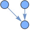
Note that each variable has a name and a distribution, and the distributions are wrapped inside Function[]. The named function variables are used to infer parent relationships between the variables.
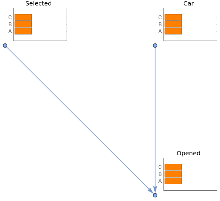
Let’s plot it:
Let’s plot it:
In[]:=
Graph[BN1,VertexLabels->"Probabilities"]
Out[]=
We can also get some information about BN:
In[]:=
Information[BN]
Out[]=
Suppose you select door A and the host opens door C. What should you do?
We can calculate the probability that the car is behind door A...
In[]:=
Probability[#Car=="A"#Selected=="A"&&#Opened=="C"&,BN1]
Out[]=
1
3
...and the probability that the car is behind door B...
In[]:=
Probability[#Car=="B"#Selected=="A"&&#Opened=="C"&,BN1]
Out[]=
2
3
We can also plot it :
In[]:=
Graph[BN1,#Selected=="A"&&#Opened=="C"&,VertexLabels->"Probabilities"]
Out[]=
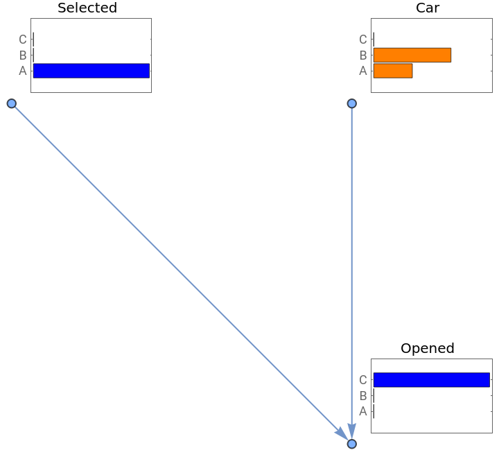
Clearly, the best choice is to switch door to B!
BNs with symbolic probabilities
BNs with symbolic probabilities
The following “wet grass” problem is commonly used to teach BNs:
In[]:=
BN2=BayesianNetwork[{<|"Name"->"Cloudy","Distribution"->Function[CategoricalDistribution[{"True","False"},{0.5,0.5}]]|>,<|"Name"->"Rain","Distribution"->Function[CategoricalDistribution[{"True","False"},Boole[#Cloudy=="True"]{0.8,0.2}+Boole[#Cloudy=="False"]{0.2,0.8}]]|>,<|"Name"->"Sprinkler","Distribution"->Function[CategoricalDistribution[{"On","Off"},Boole[#Cloudy=="True"]{0.1,0.9}+Boole[#Cloudy=="False"]{0.5,0.5}]]|>,<|"Name"->"Grass","Distribution"->Function[CategoricalDistribution[{"Wet","Dry"},Boole[#Rain=="True"&&#Sprinkler=="On"]{0.99,0.01}+Boole[#Rain=="False"&&#Sprinkler=="On"]{0.9,0.1}+Boole[#Rain=="True"&&#Sprinkler=="Off"]{0.9,0.1}+Boole[#Rain=="False"&&#Sprinkler=="Off"]{0.0,1.0}]]|>}]
Out[]=
BayesianNetwork
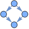
Let’s plot it:
In[]:=
Graph[BN2,#Cloudy=="True"&,VertexLabels->"Probabilities"]
In this case we may not be confident about the probability values, and maybe we want to keep some of them symbolic:
We can then investigate what happens when we change p and q:
We could even make all probabilities symbolic and make some advanced query:
Let' s ask a simple question :
...and a more complicated question:
The ability to ask such complicated questions and to mix symbolic and numeric probabilities is something I have never seen in other BN implementations or commercial tools.
How it works
How it works
Here is all the code I used to implement the paclet:
Concluding remarks
Concluding remarks
I’m quite happy that I was able to implement BNs in WL with such a small amount of code. Also, this implementation is the only one I know of that works with symbolic probabilities, which is sometimes convenient when I’m not confident enough to assign a number. With this implementation I can still perform inference and investigate how the answer varies as I change parameters. Also, the types of queries I can ask are more advanced than what I have seen in other implementations.
Of course there are also limitations. Most notably, the probability calculations becomes very slow as soon as one goes beyond small “toy examples” like I presented here. However, this is not surprising given that I haven’t implemented any efficient BN inference algorithms and solely rely on the inbuilt Probability function to do the calculations. One could possibly write new methods for Probability to mitigate this.
I hope the Wolfram will include support for BNs in the future so that my paclet becomes redundant, for example as an update to CategoricalDistribution. In the meantime, I would be interested to hear from others who have tried to implement BNs in the WL.
CITE THIS NOTEBOOK
CITE THIS NOTEBOOK
Bayesian Networks paclet: symbolic probabilities and categorical distribution support
by Andreas Hafver
Wolfram Community, STAFF PICKS, August 15, 2025
https://community.wolfram.com/groups/-/m/t/3530456
by Andreas Hafver
Wolfram Community, STAFF PICKS, August 15, 2025
https://community.wolfram.com/groups/-/m/t/3530456