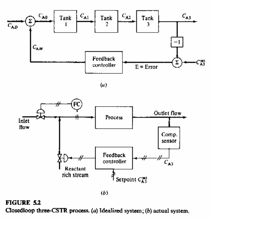
We look at the feedback control of the three CSTRs system given in the figure below (Fig. 5.2 of Ref. 1).
In the block diagram, CAD represents the disturbance concentration while CAM is the manipulated variable that is changed by the PI controller. The controller makes adjustments in order to keep CA3 (i.e., the exit concentration of tank 3 - the controlled variable) equal to its set point value (i.e., CA3set = 0.1).
In the block diagram, CAD represents the disturbance concentration while CAM is the manipulated variable that is changed by the PI controller. The controller makes adjustments in order to keep CA3 (i.e., the exit concentration of tank 3 - the controlled variable) equal to its set point value (i.e., CA3set = 0.1).
First, we find the initial values of CA1, CA2 and CA3 when CD=0 and CAM=0.8 (i.e., the nominal value or CAM(@t=0) or when the error is nil). Such calculation yields: CA1(t=0) = 0.4, CA2(t=0) = 0.2 and CA3(t=0) = 0.1.
Then, we successfully reject the disturbance (we set CAD=0.2) using a PI controller.
Then, we successfully reject the disturbance (we set CAD=0.2) using a PI controller.
To do so, we adopt two approach:
1- direct calculation based on NDSolve
2- computation based on transfer functions and block diagram
1- direct calculation based on NDSolve
2- computation based on transfer functions and block diagram
We find quantitative agreement between the two above solution approaches.
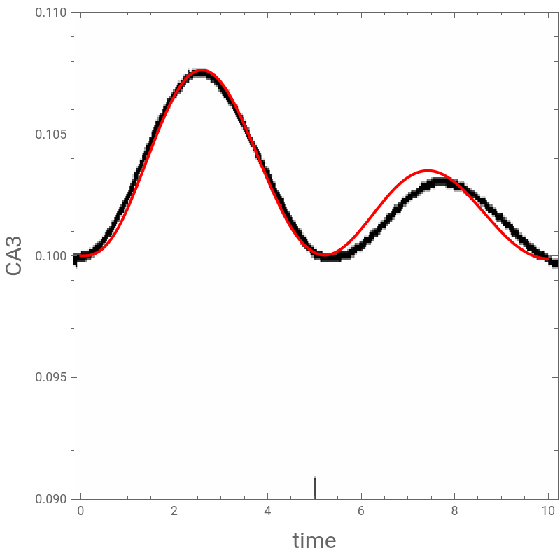
Finally, we compare our results with their counterparts given in Ref. 1.
Finally, we compare our results with their counterparts given in Ref. 1.
In[]:=
CA0[t]=CAM[t]+CAD
Out[]=
CAD+CAM[t]
In[]:=
err[t]=CA3set-CA3[t](*error*)
Out[]=
CA3set-CA3[t]
In[]:=
CAM[t]=0.8+KC(err[t]+1/TAUIIntErr[t])(*manipulatedvariable*)
Out[]=
0.8+KCCA3set-CA3[t]+
IntErr[t]
TAUI
Initial values for CA1, CA2 and CA3 when CAD = 0 and CAM = CA0 = 0.8
Parameters given in problem statement:
TAU=2;(*residencetime*)K=0.5;(*reactionrateconstant*)KC=30;(*controllergain*)TAUI=5;(*integraltimeconstant*)CA3set=0.1;(*setpoint*)CAD=0.2;(*disturbance-astepfunction*)
In[]:=
NSolve[{0==(0.8-CA1)/TAU-KCA1,0==(CA1-CA2)/TAU-KCA2,0==(CA2-CA3)/TAU-KCA3},{CA1,CA2,CA3}]//Flatten
Out[]=
{CA10.4,CA20.2,CA30.1}
In[]:=
CA0[t]
Out[]=
1.+300.1-CA3[t]+
IntErr[t]
5
In[]:=
CAM[t]
Out[]=
0.8+300.1-CA3[t]+
IntErr[t]
5
In[]:=
err[t]
Out[]=
0.1-CA3[t]
The direct approach is based on NDSolve
In[]:=
SYS={CA1'[t]==(CA0[t]-CA1[t])/TAU-KCA1[t],CA2'[t]==(CA1[t]-CA2[t])/TAU-KCA2[t],CA3'[t]==(CA2[t]-CA3[t])/TAU-KCA3[t],CA1[0]==0.4,CA2[0]==0.2,CA3[0]==0.1,IntErr'[t]==err[t],IntErr[0]==0}
Out[]=
[t]-0.5CA1[t]+1.-CA1[t]+300.1-CA3[t]+,[t](CA1[t]-CA2[t])-0.5CA2[t],[t](CA2[t]-CA3[t])-0.5CA3[t],CA1[0]0.4,CA2[0]0.2,CA3[0]0.1,[t]0.1-CA3[t],IntErr[0]0
′
CA1
1
2
IntErr[t]
5
′
CA2
1
2
′
CA3
1
2
′
IntErr
In[]:=
Length@SYS
Out[]=
8
In[]:=
UNKNOWNS={CA1,CA2,CA3,IntErr}
Out[]=
{CA1,CA2,CA3,IntErr}
In[]:=
Length@UNKNOWNS
Out[]=
4
In[]:=
SOL=NDSolve[SYS,UNKNOWNS,{t,0,50},StartingStepSize1/100,Method{"FixedStep",Method"ExplicitEuler"}]
Out[]=
CA1InterpolatingFunction,CA2InterpolatingFunction,CA3InterpolatingFunction,IntErrInterpolatingFunction


In[]:=
Plot[CA3[t]/.SOL,{t,0,50},PlotRange->{0.09,0.115},FrameLabel->{Style["time",16],Style["CA3",16]},Frame->True,GridLines->Automatic,AspectRatio->1,PlotStyle->Red]
Out[]=
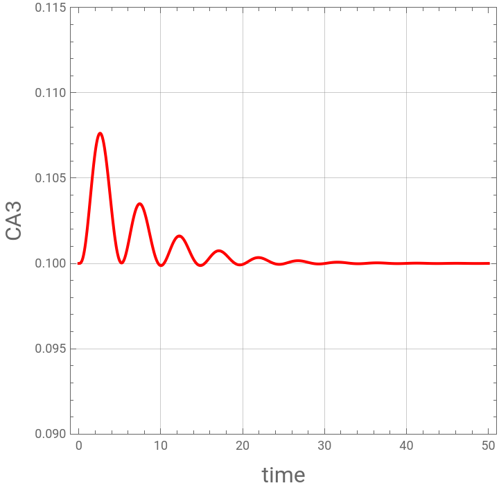
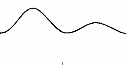
Comparison of our CA3 and the plot given in Figure 5.3 of Ref. 1
In[]:=
img=
;
In[]:=
A3=Plot[CA3[t]/.SOL,{t,0,10},PlotRange->{0.09,0.11},Frame->True,GridLines->Automatic,AspectRatio->1,PlotStyle->Red,FrameLabel->{Style["time",16],Style["CA3",16]}];
In[]:=
Show[A3,ImageSize400{1,1},Prolog{Raster[ImageData[img,DataReversedTrue],{Scaled[{0.005,0.00}],Scaled[{1,1}]}]}]
Out[]=
The second approach is based on transfer functions and block diagram
In[]:=
Gp=1/(TAUs+1+KTAU)^3
Out[]=
1
3
(2.+2s)
In[]:=
Gc=KC(1+1/s/TAUI)
Out[]=
301+
1
5s
In[]:=
G=Gp/(1+GpGc)//Expand//FullSimplify
Out[]=
0.125s
0.75+s(4.75+s(3.+s(3.+s)))
In[]:=
Roots[0.75`+s(4.75`+s(3.`+s(3.`+s)))==0,s](*allrootsofthesystem'scharacterisiticequationhavenegativerealpart-wegetastableresponse*)
Reproducing the numerical values given in Table 5.4 of Ref. 1
References
References
[1] W. L. Luyben, Process Modelling, Stimulation and Control for Chemical Engineers, 2nd Edition, NY: McGraw-Hill, 1996
CITE THIS NOTEBOOK
CITE THIS NOTEBOOK
PI control of three CSTRs in series
by Housam Binous and Ahmed Bellagi
Wolfram Community, STAFF PICKS, November 10, 2024
https://community.wolfram.com/groups/-/m/t/3317070
by Housam Binous and Ahmed Bellagi
Wolfram Community, STAFF PICKS, November 10, 2024
https://community.wolfram.com/groups/-/m/t/3317070