Space travel requires high degrees of precision due to the vast distances traveled and cumulative effects of even miniscule effects over long durations. This essay explores an in depth visualization and quantification of the two most significant factors for orbit decay: J2 perturbation and atmospheric drag. Beyond addressing long term decay, we also investigate the short term effects of these perturbations in real maneuvers like the Hohmann Transfer. This project deepens understanding of orbit decay with visualizations and supports that satellites need constant monitoring, as the simulated Hohmann transfer had deviated from theoretical values by over 500km after only 2 hours. Finally, with a combination of Newtonian and Lagrangian mechanics, we examine how further deformation of Earth would affect the gravitational field and orbits.
Introduction
Introduction
The study of orbital dynamics seeks to understand how objects move under the influence of gravity and other forces in space. In particular, Earth’s oblate shape causes a phenomenon known as the J2 perturbation, where the planet’s equatorial bulge distorts its gravitational field and gradually alters the orientation of the orbital plane. Furthermore, low-Earth orbit (LEO) satellites must contend with atmospheric drag—a force caused by collisions with residual atmospheric particles—which leads to orbital decay over time. In this project, we will investigate how both J2 perturbation and atmospheric drag impact the stability, altitude, and precession of satellite orbits. By simulating these perturbations over short and long periods of time, we will try to better understand orbital drift and develop insights into long-term satellite behavior and mission planning.
Newtonian Mechanics
Newtonian Mechanics
Newtonian mechanics, also known as classical mechanics, is the branch of physics that describes the motion of objects under the influence of forces. It is dictated by the famous equation F = ma, which states that the force exerted upon an object is equal to the product of its mass and acceleration. According to Newtonian Mechanics, the force of gravity is F = , where M and m are masses, r is the distance, and G is the gravitational constant, although μ is often substituted for GM, which is called the gravitational parameter. The idea of approaching physics from a force perspective is important, as we will later view physics from an energy perspective, which can have many benefits.Following standard physics conventions, the following units will be used in this project: meters (m), kilograms (kg), and seconds (s).
GMm
2
r
Generating Gravitational Fields
Generating Gravitational Fields
Define constants and Earth’s oblate shape (in SI units).
G=6.6743×10^-11; earthMass=5.97219×10^24;{r1, r2, r3}={6378000, 6378000,6357000};μ = G*earthMass;
Plot a spherical Earth’s gravitational force for comparison.
ShowSliceDensityPlot3Dμ(x^2+y^2+z^2),"CenterPlanes",{x,-2r1,2r1},{y,-2r2,2r2},{z,-2r3,2r3}, RegionFunction->Function[{x,y,z},!RegionMember[Ellipsoid[{0,0,0},{r1,r2,r3}],{x,y,z}]], Graphics3D[Ellipsoid[{0,0,0},{r1,r2,r3}]]
Out[]=
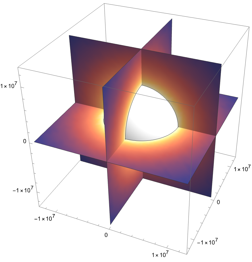
Newton’s Shell Theorem lets us assume constant density because Earth’s density comes in layers: inner core, outer core, mantle, and crust. That means the non-uniform density distribution will have minimal impact on orbits.
Set density to (kg/)
M
E
V
E
3
m
In[]:=
ρ=earthMass/((4/3)*Pi*r1*r2*r3);
Define two functions to model gravitational force (oblate Earth, and ideal Earth).
accelGravityEllipse2d[x_?NumericQ,y_?NumericQ]:= -NIntegrate[(G*ρ/((x-p1)^2+(y-p2)^2))*Normalize[{(x-p1),(y-p2)}],{p1,p2}∈Ellipsoid[{0,0},{r1,r3}]]accelGravityCircle2d[x_?NumericQ,y_?NumericQ]:= -NIntegrate[(G*ρ/((x-p1)^2+(y-p2)^2))*Normalize[{(x-p1),(y-p2)}],{p1,p2}∈Ellipsoid[{0,0},{(r1+r3)/2,(r1+r3)/2}]]
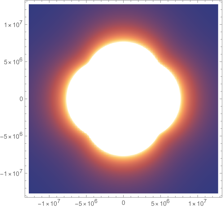
Visualize the difference between an oblate and ideal model of Earth.
QuietDensityPlotNorm[accelGravityEllipse2d[x,y]-accelGravityCircle2d[x,y]],{x,-2r1,2r1},{y,-2r3,2r3}, PlotPoints->80,RegionFunction->Function[{x,y},!RegionMember[Ellipsoid[{0,0},{r1,r3}],{x,y}]]
Out[]=
ShowVectorPlotaccelGravityEllipse2d[x,y]-accelGravityCircle2d[x,y],{x,-2r1,2r1},{y,-2r1,2r1}, VectorScaling->Automatic,RegionFunction->Function[{x,y},!RegionMember[Ellipsoid[{0,0},{r1,r3}],{x,y}]]
Out[]=
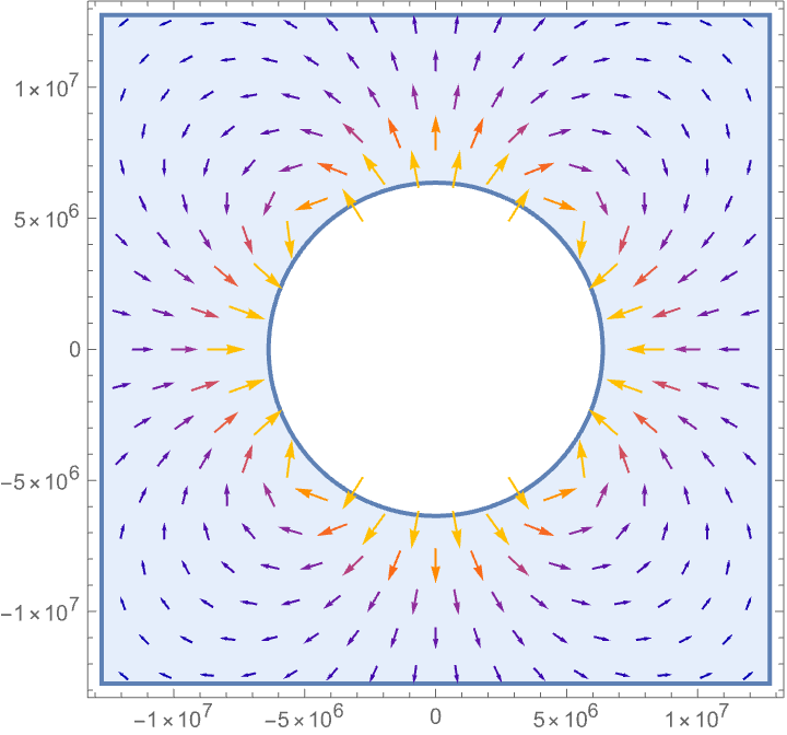
There are clearly some unusual artifacts, particularly near Earth’s equator and poles. These arise from the nonuniform vector field caused by Earth’s oblate shape. Let’s now explore how this distorted gravitational field influences the orbits around Earth.
Modeling Orbits Around Earth
Modeling Orbits Around Earth
Start with a point mass scenario.
In[]:=
pointGravity[x_,y_,z_]:=((-G)*earthMass/(x^2+y^2+z^2))*Normalize[{x,y,z}];
Initial conditions of orbit (m).
In[]:=
initialPosition={7000000,0,0};initialVelocity={0,7600,0};
Solve the second order differential equation.
In[]:=
eqnsOfMotion=x''[t]==(pointGravity[x,y,z][[1]]/.{x->x[t],y->y[t],z->z[t]}), y''[t]==(pointGravity[x,y,z][[2]]/.{x->x[t],y->y[t],z->z[t]}), z''[t]==(pointGravity[x,y,z][[3]]/.{x->x[t],y->y[t],z->z[t]}), x[0]==initialPosition[[1]],y[0]==initialPosition[[2]],z[0]==initialPosition[[3]], x'[0]==initialVelocity[[1]],y'[0]==initialVelocity[[2]],z'[0]==initialVelocity[[3]];
Extract parametrized functions.
In[]:=
{xFunc,yFunc,zFunc}=NDSolveValue[eqnsOfMotion,{x,y,z},{t,0,15000,1}];trajectoryData=Table[{xFunc[t],yFunc[t],zFunc[t]},{t,0,15000,1}];
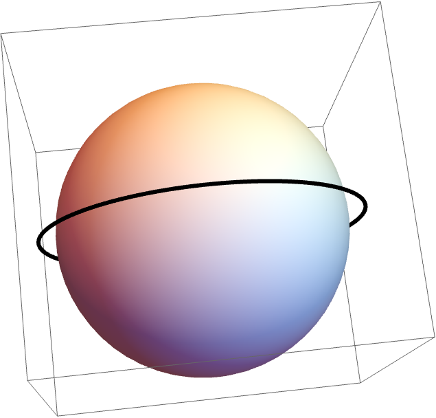
Plot the orbit.
ShowGraphics3D[Sphere[{0,0,0},r1]], Graphics3D[{AbsoluteThickness[3],Line[trajectoryData]}]
Out[]=
Create a new function to model gravitational force while taking Earth’s oblate shape into account.
Define initial position (m) and velocity (m/s).
4th Order Runge-Kutta ODE Solver
4th Order Runge-Kutta ODE Solver
During my process, I was unfortunately unable to use NDSolve with our new gravity function to solve for a position vector like I did with the point mass, which was most likely due to compatibility issues with NIntegrate and NDSolve. I instead made a differential equation solver using the Runge Kutta method (RK4). RK is essentially a more complex Euler’s method; in one timestep, n number of points are sampled and evaluated. Then, by taking a weighted average of these slopes, the next point is found. In my solver, I sampled 4 points (start, end, and two in the middle), so it is a 4th order Runge Kutta function (Weisstein).
Run the solver.
Plot the orbit. This orbit has a high inclination orbit of 45 degrees.
Define a (m).
Check the period (s).
Our calculated period is equivalent to the period of the orbit generated by our solver, so it is accurate.
Effects of Earth’s Nonuniform Gravitational Field on a Hohmann Transfer
Effects of Earth’s Nonuniform Gravitational Field on a Hohmann Transfer
Now that we can model Earth’s gravitational fields and plot orbits, we can try applying these tools to some real scenarios. One frequently used space maneuver is the Hohmann Transfer. In this transfer, a satellite starts at a lower initial circular orbit and burns to speed up. With more speed, the orbital path becomes elliptical, and when the satellite is at the apogee (furthest point in the orbital path), it performs a second burn to correct its velocity and restore a circular orbit. Effectively, with two precise thrusts, a satellite can transfer from a low earth orbit (LEO) to a medium (MEO) or geostationary earth orbit (GEO).
Define our starting and ending orbits (roughly circular). We will start at 122km altitude and transfer to a 13622km altitude orbit.
The two thrusts and transit time are given by (Lynnane):
Calculate the two thrusts and
Find mass loss (kg).
Modify our RK4 solver to implement these two burns.
Run the solver.
Plot the orbit.
Above, green is the initial orbit, red is the elliptical transfer orbit, and blue is the final orbit.
Lets compare our measured values to the theoretical value at the black point, which should be when the satellite transfers to the higher orbit.
Now subtract the two.
Quantify these numbers in percentages.
The position and velocities are off by 2-3%, and the direction of the satellite is off by ~1.3 degrees. In raw numbers for our transfer, the position was off by over 500km and the speed was off by ~100m/s. This deviation occurred only after ~2.4 hours, thus highlighting the importance of constant satellite maintenance.
Lagrangian Mechanics
Lagrangian Mechanics
Diagram of equatorial plane (gray) and orbital plane (yellow) with four rotation-describing elements (Wikipedia)
Orbit Decay/Drift Over Extended Periods of Time
Orbit Decay/Drift Over Extended Periods of Time
Define the J2 constant (dimensionless).
Initial position (m) and velocity (m/s).
Functions for eccentricity (e) and inclination (i). The semi-major axis was defined above (a).
Evaluating initial conditions of orbital plane: semi-minor axis (b), period (t), mean motion (n), and semi-latus rectum (p).
Lagrange’s planetary equations are a system of differential equations for each orbital element. The equations for Ω and ω are below, where R is the perturbing function (Murray & Dermott).
This can all be simplified, though, especially because we are considering the other four elements as constants. We are eventually left with cleaner expressions for J2 perturbation on the mean orbital elements:
Define our differential equation system.
Use NDSolve to find position functions.
Create an animation to visualize orbital drift.
This is how the orbit trajectory would evolve over 500 rotations (~1.78 hours/rotation). Secular drift are the changes that happen slowly over time, like demonstrated above with J2. On the other hand, orbits also experience both short and long period oscillating effects, such as the periodic shift of ocean tides.
Explorations of Deformed Earths
Explorations of Deformed Earths
Now that we are able to model secular effects in orbit trajectories, lets see how deforming the Earth affects orbits. Although this section isn’t very realistic, I’ll look at two scenarios of Earth with different shapes.
Fat Earth
Fat Earth
A simple example to start. Basically an exaggerated version of the J2 perturbation.
Define new shape. The horizontal cross section radius is doubled.
Model the new Earth.
Calculate J2 (dimensionless).
Define initial variables (in SI units).
Solve differential equations.
Create the model. Notice that the range of the slider is changed to only one period, due to how much faster the orbit shifts.
This animation makes sense; a wider Earth leads to a higher J2, and vice versa.
Banana Earth
Banana Earth
Inspired by Gregory, lets take a quick look at orbits around a banana-shaped Earth.
Create the banana.
Due to the complex region, we will instead sample 1000 points in the banana.
Differential equations for orbit.
Plot the orbit.
Surprisingly, we can still notice a similar drift in orbit. It starts at the black point and its orbital plane is angled towards the top left. As it orbits, the plane rotates counterclockwise, similar to our Lagrangian models above.
Conclusion
Conclusion
In this project, we examined how Earth’s oblate shape affects orbital paths over time. These secular drifts were prevalent in the right ascension of the ascending node and argument of periapsis. On the other hand, we also examined the short term effects of J2 perturbing forces and atmospheric drag. We were able to find that over the course of a few hours only, orbits deviate significantly from their expected values if left unattended, as shown with the simulated Hohmann Transfer (>500km off). Finally, we examined different shapes of celestial bodies and noticed similar trends between them. This project contributes to not just the quantification, but also the visualization of perturbing forces on orbits, the latter being rather significant as it is a step towards a better understanding of space travel and our planet.
Limitations and Future Work
Limitations and Future Work
Citations
Citations
◼
Moritz, H. (2000). Geodetic Reference System 1980. Retrieved from https://ciencias.ulisboa.pt/sites/default/files/fcul/dep/dqb/doc/GRS80_Moritz.pdf
◼
Baratta, A., & others. (2024). General relativity and satellite motion: A Newtonian-like formulation and its applications [Preprint]. arXiv. https://arxiv.org/abs/2405.18140
◼
Murray, C. D., & Dermott, S. F. (n.d.). Solar System Dynamics (Chapter 6). Retrieved from https://adams.dm.unipi.it/~bau/PDF/didattica/2023_24/DSS/MurrayDermott_cap6.pdf
◼
Lynnane, G. (n.d.). Chapter 7: Maneuvering. In Introduction to Aeronautics. Open Education Resource. https://oer.pressbooks.pub/lynnanegeorge/chapter/chapter-7-manuvering/
◼
Brennen, C. E. (2005). Rocket propulsion (Ch. 4). In Fundamentals of Multiphase Flow. Retrieved from http://brennen.caltech.edu/fluidbook/externalflows/propulsion/rocketpropulsion.pdf
◼
Wolfram Demonstrations Project. (n.d.). The effect of the spherical harmonic gravitational potential on satellite motion. Retrieved from https://demonstrations.wolfram.com/TheEffectOfTheSphericalHarmonicGravitationalPotentialOnSatel/
◼
Prussing, J. E., & Conway, B. A. (1993). Orbital mechanics. New York, NY: Oxford University Press.
◼
Orbital elements. (2025, July 4). In Wikipedia. Retrieved July 10, 2025, from https://en.wikipedia.org/wiki/Orbital_elements
◼
NASA Glenn Research Center. (n.d.). Drag equation. In Beginner’s guide to aeronautics – K‑12. Retrieved July 10, 2025, from https://www.grc.nasa.gov/www/k-12/VirtualAero/BottleRocket/airplane/drageq.html
◼
Weisstein, E. W. (n.d.). Runge–Kutta method. In MathWorld–A Wolfram Web Resource. Retrieved July 10, 2025, from https://mathworld.wolfram.com/Runge-KuttaMethod.html
Acknowledgements
Acknowledgements
I would like to thank my mentor Shenghui Yang for supporting my exploration and research of my interests at the WRSP program. Beyond a mentor, Shenghui and our mentor group have made the research process not just informative, but also fun and enjoyable. Final thanks to Program Director Rory Foulger, Academic Director Eryn Gillam, Academic Director Megan Davis, and all of the TAs for a great experience.
CITE THIS NOTEBOOK
CITE THIS NOTEBOOK
Visualizing orbital decay due to Earth's oblate shape
by Alex Ning
Wolfram Community, STAFF PICKS, July 11, 2025
https://community.wolfram.com/groups/-/m/t/3502450
by Alex Ning
Wolfram Community, STAFF PICKS, July 11, 2025
https://community.wolfram.com/groups/-/m/t/3502450