Wolfram Cloud Document

Gas Constant expressed in kcal/kmol*K and Pressure expressed in mmHg

In[]:=

R=1.987;P=760;

Activity coefficients using NRTL model
Component 1 = 1-Butanol
Component 2 = Water

In[]:=

Gam[i_]:=Exp

∑

j=1

(t[j,i]G[j,i]x[j])

∑

l=1

(G[l,i]x[l])

∑

j=1

G[i,j]x[j]

∑

l=1

(G[l,j]x[l])

t[i,j]-

∑

r=1

(t[r,j]G[r,j]x[r])

∑

l=1

(G[l,j]x[l])

/.x[1]x1/.x[2]1-x1

In[]:=

Gamp[i_]:=Exp

∑

j=1

(t[j,i]G[j,i]x[j])

∑

l=1

(G[l,i]x[l])

∑

j=1

G[i,j]x[j]

∑

l=1

(G[l,j]x[l])

t[i,j]-

∑

r=1

(t[r,j]G[r,j]x[r])

∑

l=1

(G[l,j]x[l])

/.x[1]xp1/.x[2]1-xp1

In[]:=

G[i_,j_]:=Exp[-a[i,j]t[i,j]]

In[]:=

t[i_,j_]:=g[i,j]/(R(T+273.15))

Binary interaction parameters and non-randomness factors are taken from Aspen-HYSYS

g[1,1]=0;g[2,2]=0;g[2,1]=2794.6660;g[1,2]=570.13620;a[1,1]=0;a[2,2]=0;a[1,2]=0.47;a[2,1]=0.47;

Vapor Pressure Using Antoine Equation

In[]:=

A1=7.36366;B1=1305.198;C1=173.427;

In[]:=

A2=8.07131;B2=1730.630;C2=233.426;

In[]:=

PS1=10^(A1-B1/(C1+T));PS2=10^(A2-B2/(C2+T));

Normal boiling temperatures

In[]:=

FindRoot[PS1P,{T,100,120}]

Out[]=

{T117.727}

In[]:=

FindRoot[PS2P,{T,100,120}]

Out[]=

{T99.9968}

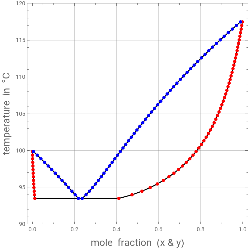
Heterogeneous Azeotrope (overall liquid composition 22.6 mole % and b.p. 93.24 °C)

In[]:=

FindRoot[{y1Gam[1]x1PS1/P,Gam[1]x1PS1/PGamp[1]xp1PS1/P,Gamp[1]xp1PS1+Gamp[2](1-xp1)PS2P,Gam[1]x1PS1+Gam[2](1-x1)PS2P},{x1,0.005,0.01},{xp1,0.35,0.4},{y1,0.2,0.25},{T,90,95}]

Out[]=

{x10.0124991,xp10.366001,y10.226053,T93.2468}

Computing VLE data

In[]:=

i=0;

In[]:=

While[i<101,{T=Evaluate[93.2468+i(117.727-93.2468)/100],Temp[i]=T,x1[i]=FindRoot[{Gam[1]x1PS1+Gam[2](1-x1)PS2P},{x1,0.3,0.95}][[1,2]],xp1[i]=FindRoot[{Gam[1]x1PS1+Gam[2](1-x1)PS2P},{x1,0.005,0.01}][[1,2]],y1[i]=Gam[1]x1PS1/P/.x1x1[i],yp1[i]=Gam[1]x1PS1/P/.x1xp1[i],i++}]

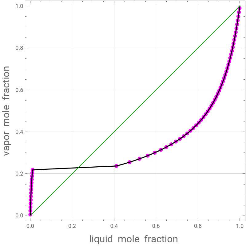
T-xy and xy plots for the 1-Butanol - water system

In[]:=

tb1=Table[{x1[i],Temp[i]},{i,1,100,2}];

In[]:=

tb2=Table[{xp1[i],Temp[i]},{i,1,27,2}];

In[]:=

tb3=Table[{y1[i],Temp[i]},{i,1,100,2}];

In[]:=

tb4=Table[{yp1[i],Temp[i]},{i,1,27,2}];

In[]:=

tbf1=Sort[Join[tb1,tb2]];

In[]:=

tbf2=Sort[Join[tb3,tb4]];

In[]:=

plt1=ListPlot[tbf1,PlotStyle{RGBColor[1,0,0],PointSize[0.015]},PlotRange{{-0.2,1.2},{90,120}}];

In[]:=

plt2=ListPlot[tbf2,PlotStyle{RGBColor[0,0,1],PointSize[0.015]},PlotRange{{-0.2,1.2},{90,120}}];

In[]:=

plt1b=ListPlot[tbf1,PlotStyleRGBColor[0,0,0],PlotRange{{-0.2,1.2},{90,120}},JoinedTrue];

In[]:=

plt2b=ListPlot[tbf2,PlotStyleRGBColor[0,0,0],PlotRange{{-0.2,1.2},{90,120}},JoinedTrue];

In[]:=

a1=Show[plt1b,plt2b,plt1,plt2,FrameTrue,GridLinesAutomatic,PlotRange{{-0.025,1.025},{90,120}},ImageSize400{1,1},FrameLabel{Style["mole fraction (x & y)",16],Style["temperature in °C",16]},AspectRatio1]

Out[]=

In[]:=

tb5=Table[{x1[i],y1[i]},{i,1,100,2}];

In[]:=

tb6=Table[{xp1[i],yp1[i]},{i,1,27,2}];

In[]:=

tbf3=Sort[Join[tb5,tb6]];

In[]:=

plt3=ListPlot[tbf3,PlotStyle{Magenta,PointSize[0.0175]},FrameTrue,GridLinesAutomatic,PlotRange{{-0.025,1.025},{-0.025,1.025}},ImageSize400{1,1},FrameLabel{Style["liquid mole fraction ",16],Style["vapor mole fraction",16]},AspectRatio1];

In[]:=

tb5=Table[{x1[i],y1[i]},{i,1,100}];

In[]:=

tb6=Table[{xp1[i],yp1[i]},{i,1,27}];

In[]:=

tbf3=Sort[Join[tb5,tb6]];

In[]:=

plt3b=ListPlot[tbf3,PlotStyleRGBColor[0,0,0],JoinedTrue,FrameTrue,GridLinesAutomatic,PlotRange{{-0.025,1.025},{-0.025,1.025}},ImageSize400{1,1},FrameLabel{Style["liquid mole fraction ",16],Style["vapor mole fraction",16]},AspectRatio1];

In[]:=

a2=Show[plt3,plt3b,Epilog{Darker@Green,Line[{{0,0},{1,1}}]}]

Out[]=

Comparing with data from either Ref. 5 or Ref. 6 (displayed by green squares)

In[]:=

DATACHU={{x_water,y_water,Tboiling},{0.,0.,117.},{3.9,26.7,111.5},{4.7,29.9,110.6},{5.5,32.3,109.6},{7.0,35.2,108.8},{25.7,62.9,97.9},{27.5,64.1,97.2},{29.2,65.5,96.7},{30.5,66.2,96.3},{49.6,73.6,93.5},{50.6,74.0,93.4},{55.2,75.0,92.9},{56.4,75.2,92.9},{57.1,74.8,92.9},{57.3,75.0,92.8},{97.5,75.2,92.7},{98.0,75.6,93.0},{98.2,75.8,92.8},{98.5,77.5,93.4},{98.6,78.4,93.4},{98.8,80.8,93.7},{99.2,84.3,95.4},{99.4,88.4,96.8},{99.7,92.9,98.3},{99.8,95.1,98.4},{99.9,98.1,99.4},{100.,100.,100.}};

In[]:=

DATACHU//TableForm

Out[]//TableForm=

x_water	y_water	Tboiling
0.	0.	117.
3.9	26.7	111.5
4.7	29.9	110.6
5.5	32.3	109.6
7.	35.2	108.8
25.7	62.9	97.9
27.5	64.1	97.2
29.2	65.5	96.7
30.5	66.2	96.3
49.6	73.6	93.5
50.6	74.	93.4
55.2	75.	92.9
56.4	75.2	92.9
57.1	74.8	92.9
57.3	75.	92.8
97.5	75.2	92.7
98.	75.6	93.
98.2	75.8	92.8
98.5	77.5	93.4
98.6	78.4	93.4
98.8	80.8	93.7
99.2	84.3	95.4
99.4	88.4	96.8
99.7	92.9	98.3
99.8	95.1	98.4
99.9	98.1	99.4
100.	100.	100.

Computing LLE data

We reproduce the figure below, which was given by Doherty et al. (Ref. 4). Minor discrepancies are most likely due to different thermodynamic data (i.e., NRTL and Antoine constants)

References

◼

J. M. Smith, H. C. Van Ness and M. M. Abbott, Introduction to Chemical Engineering Thermodynamics, 7th ed., Boston: McGraw-Hill, 2005.

◼

H. Renon and J. M. Prausnitz, “Local Compositions in Thermodynamic Excess Functions for Liquid Mixtures,” AIChE Journal, 14(1), 1968 pp. 135–144. doi:10.1002/aic.690140124.

◼

Aspentech. “Aspen-HYSYS.” (Dec 15, 2016) www.aspentech.com/products/aspen-hysys.

◼

M. F. Doherty, Z. T. Fidkowski, M. F. Malone and R. Taylor, Distillation, Section 13, Perry’s Chemical Engineer’s Handbook, 8th edition, NY: McGraw-Hill, 2008.

◼

J. C. Chu, R. J. Getty, L. F. Brennecke, and R. Paul, Distillation Equilibrium Data, NY: Reinhold, 1950.

◼

P. C. Wankat, Separation Process Engineering: Includes Mass Transfer Analysis, 3rd edition, Upper Saddle River: Prentice Hall, 2012.

CITE THIS NOTEBOOK

Vapor-liquid and liquid-liquid equilibrium computations of a partially miscible binary system: 1-Butanol - water case
by Housam Binous & Ahmed Bellagi
Wolfram Community, STAFF PICKS, October 27, 2024
https://community.wolfram.com/groups/-/m/t/3308968