We study the one-dimensional heat conduction equation on the finite interval, subject to Dirichlet boundary conditions
u
t
u
xx
u
0
g
0
h
0
Applying the Fourier transform of both sides of the heat equation and integrating by parts twice yields the following first-order ODE in .
t
∂
u
∂t
2
λ
u
u
x
-iλ
e
u
x
We use the integrating factor method and Integrating both sides with respect to we obtain
t
2
λ
e
u
u
0
g
1
2
λ
g
0
2
λ
-λi
e
h
1
2
λ
h
0
2
λ
This is called the Global Relation (G.R). This equation is valid for all and t>0. Inverting the Fourier transform formally gives:
λ∈C
u(x,t)(λ)λ-(,t)+iλ (,t)λ+(,t)+iλ (,t)λ
1
2π
∞
∫
-∞
iλx-t
2
λ
e
u
0
1
2π
∞
∫
-∞
iλx-t
2
λ
e
g
1
2
λ
g
0
2
λ
1
2π
∞
∫
-∞
-iλ(1-x)-t
2
λ
e
h
1
2
λ
h
0
2
λ
For the first two integrals, that is the formula for the heat equation on the half-line, where the contour is the boundary of the domain defined by
∂
+
D
+
D
-
D
2
λ
We now specialise the general representation to the explicit choice of data
u
0
-x
e
g
0
h
0
-1
e
The transforms that correspond to these conditions are :
u
0
-i(1-)
-(1+iλ)
e
λ-i
g
0
λt
e
2
λ
h
0
g
0
e
The contour is taken to be the trapezoidal path defined by
+
C
z
1
3
4
i
5π
6
e
z
2
z
3
3
4
i
π
6
e
with .
ℓ
3
4
The solution reduces to a single integral:
u(x,t)-dλ
1
2π
∫
+
C
-t
2
λ
e
iλ
e
-iλ
e
Q(λ,x)·(-1)
2
λ
(+1)·(+1)
2
λ
4
λ
where
Q(λ,x)-4λ+sin(λ(1-x))
sin(λx)
e
Define the complex-valued function V(k,x,t)
v[k_,x_,t_]:=**
1
2*Pi
Exp[-k^2t]
Exp[I*k]-Exp[-I*k]
-4*k+Sin[k*(1-x)](k^2-1)
Sin[k*x]
(k^2+1)*(k^4+1)
Set L value
l=3/4;
Define the three contours k1,k2,k3
k1[r_]:=l+(3/4)*I+r*Exp[I*Pi/6];k2[r_]:=-l+(3/4)*I+r*Exp[I*5*Pi/6];k3[s_]:=s+(3/4)*I;
Derivatives of the contours
dk1[r_]:=D[k1[r],r];dk2[r_]:=D[k2[r],r];dk3[s_]:=D[k3[s],s];
Define the approxU function with NumericQ guards
approxU[x_?NumericQ,t_?NumericQ]:=Module[{temp1,temp2},temp1=NIntegrate[Re[v[k1[r],x,t]*dk1[r]-v[k2[r],x,t]*dk2[r]],{r,0,Infinity},AccuracyGoal->6,PrecisionGoal->6,MaxRecursion->20];temp2=NIntegrate[Re[v[k3[s],x,t]*dk3[s]],{s,-l,l},AccuracyGoal->6,PrecisionGoal->6,MaxRecursion->20];temp1+temp2]
Example: Evaluate at a point
approxU[0.5,0.1]
Out[]=
0.653637
Step 4: Plot the 3D surface
Plot3D[approxU[x,t],{x,0,1},{t,0,2Pi},AxesLabel->{"x","t","u(x,t)"},PlotLabel->"Fokas Method Solution of Half-Line Heat Equation",Mesh->None]
Out[]=

With{times={0.1,0.2,0.3,0.4,0.5,0.6},styles=ColorData[97,"ColorList"]},PlotEvaluate[Join[Table[approxU[x,t],{t,times}],{u[x,0]}]],{x,0,1},
Out[]=
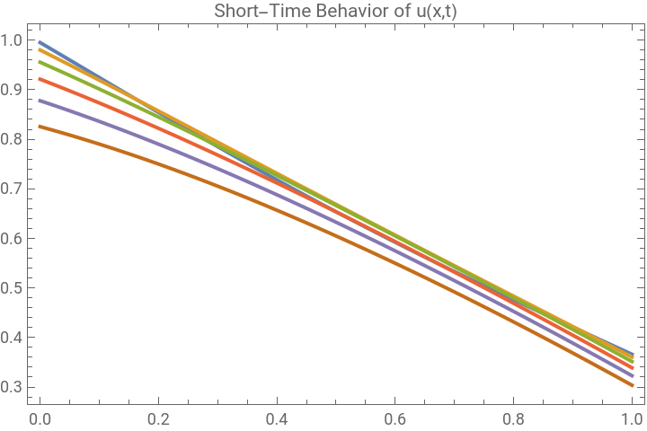


In[]:=
With[{times={0.5,1,1.5,2,2.5,3},styles=ColorData[97,"ColorList"]},Plot[Evaluate[Join[Table[approxU[x,t],{t,times}],{u[x,0]}(*Thisisu(x,0)*)]],{x,0,1},PlotStyle->Join[styles[[;;Length[times]]],(*applydistinctcolorpert*){{Black,Dashed}}(*styleforu(x,0)*)],PlotLegends->LineLegend[Join[Table["t = "<>ToString[t],{t,times}],{"u(x,0)"}],LegendLabel->"Long-Time Behavior"],AxesLabel->{"x","u(x,t)"},PlotLabel->"Long-Time Behavior of u(x,t)",Frame->True,Axes->False]]
Out[]=
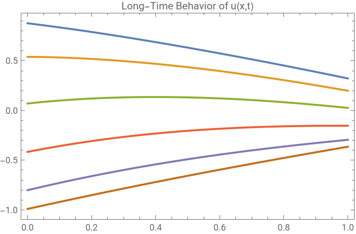
CITE THIS NOTEBOOK
CITE THIS NOTEBOOK
An introduction to the U.T.M: the heat equation on a finite interval
by Athanasios Paraskevopoulos
Wolfram Community, STAFF PICKS, August 2, 2026
https://community.wolfram.com/groups/-/m/t/3771904
by Athanasios Paraskevopoulos
Wolfram Community, STAFF PICKS, August 2, 2026
https://community.wolfram.com/groups/-/m/t/3771904