Recreating figure 1.5 from Real Sound Synthesis
Recreating figure 1.5 from Real Sound Synthesis
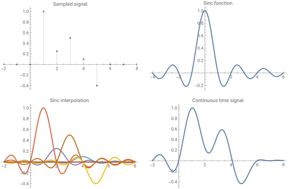
I wanted to understand the process of resampling with sinc by reconstructing figure 1.5 of the book Real Sound Synthesis for Interactive Applications by Perry R. Cook:
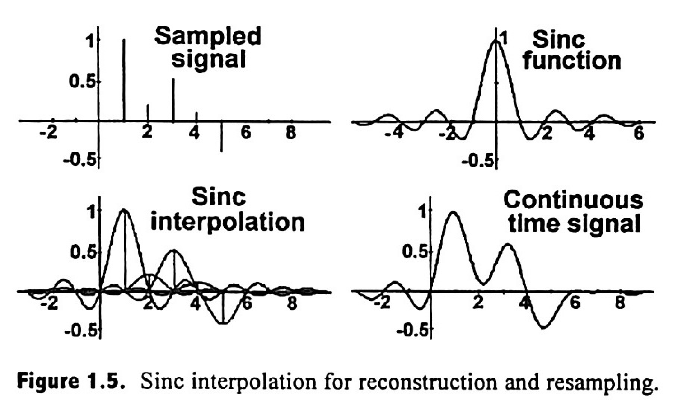
The book describes the process:
1
.Produce a continuous time signal from the samples by convolving the original signal with an appropriately-parameterized sinc function.
2
.Freely sample from that continuous signal at whatever intervals you want.
This method is “ideal in a provable digital signal processing sense” under the assumption that the original samples were made from an analog signal that had no frequency components above the Nyquist frequency (half the sample rate). When that assumption doesn’t hold, you get similar results, but frequencies above the Nyquist will be aliased as lower frequencies. Basically, it will sound distorted. If the original sampled audio sounds fine when you play it, then it’s probably been band-limited in this way.
Resampling with this method is very expensive because sinc only approaches zero in the limits at infinity. However, for this notebook, that doesn’t matter. In practical applications, you might use another convolutional kernel—perhaps even a windowed sinc.
Sinc, as defined in the book
Sinc, as defined in the book
First, I’ll define inc with the parameterization used in the book, where:- is the current time (in seconds, if you want to interpret the sample rates as Hz), and- is the sample rate of the signal being resampled.
t
sRate
Like , we define it to be 1 at 0.
In[]:=
sinc[0,_]:=1sinc[t_,sRate_]:=With[{T=1/sRate},Sin[πt/T]/(πt/T)]Plot[sinc[x,1],{x,-4,6},PlotRange->Full]
Out[]=
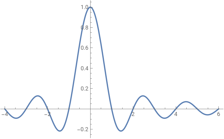
This function is 1 at and 0 at every integer . This is how it ensures that if you sample the continuous signal post-convolution, you get the original samples back, even though the function is non-zero nearly everywhere and you might otherwise expect samples to blur into one another.
t=0
t
In[]:=
Table[sinc[t,1],{t,-4,6}]
Out[]=
{0,0,0,0,1,0,0,0,0,0,0}
It was useful for me to explore the shapes sinc can take on as we manipulate all the parameters we need to perform the convolution:
In[]:=
Manipulate[Plot[amplitude*sinc[(x-x0),sRate],{x,-2,8},PlotRange->{-1,1}],{{amplitude,1},0,1},{{x0,0},-2,8},{{sRate,1},0.00001,2},SaveDefinitions->True]
Out[]=


Define the fake audio signal
Define the fake audio signal
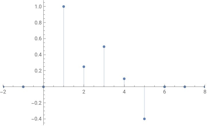
Here, I define the audio samples shown in figure 1.5. I estimated each sample’s amplitudes by eyeballing the chart.
In[]:=
samples={{-2,0},{-1,0},{0,0},{1,1},{2,.25},{3,.5},{4,.1},{5,-.4},{6,0},{7,0},{8,0}};ListPlot[samples,Filling->Axis,PlotRange->{{-2,8},Automatic}]
Out[]=
Produce a continuous time signal from the samples
Produce a continuous time signal from the samples
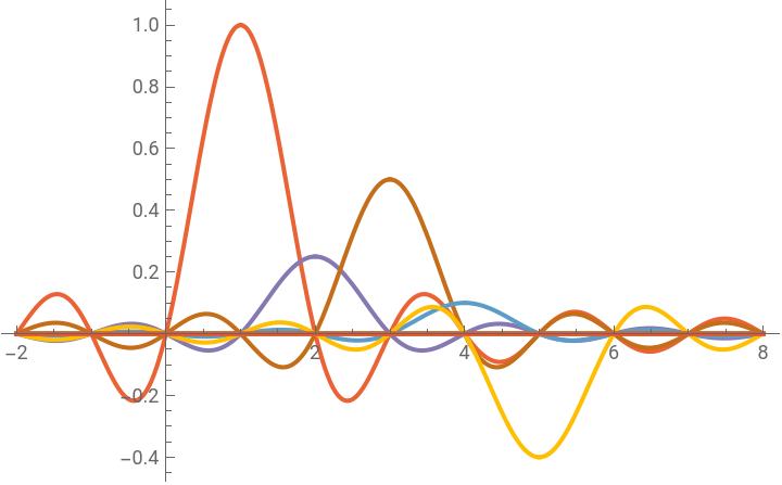
First, I convolve every sample with sinc individually, recreating the bottom left chart in figure 1.5.
In[]:=
sincs=Map[sample|->sample[[2]]*sinc[(t-sample[[1]]),1],samples];Plot[sincs,{t,-2,8},PlotRange->Full]
Out[]=
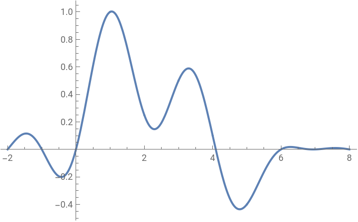
Then, I plot their sum, which is the final continuous signal. This is the function you would sample from at whatever new rate you choose.
In[]:=
Plot[Total[sincs],{t,-2,8},PlotRange->Full]
Out[]=
Finally, recreate the figure in the book
Finally, recreate the figure in the book
All together, just like in the book:
In[]:=
GraphicsGrid[{{ListPlot[samples,Filling->Axis,PlotRange->{{-2,8},Automatic},PlotLabel->"Sampled signal"],Plot[sinc[x,1],{x,-4,6},PlotRange->Full,PlotLabel->"Sinc function"]},{Plot[sincs,{t,-2,8},PlotRange->Full,PlotLabel->"Sinc interpolation"],Plot[Total[sincs],{t,-2,8},PlotRange->Full,PlotLabel->"Continuous time signal"]}}]
Out[]=
Explore a bit further
Explore a bit further
For my own edification, I wanted to overlay the sampled and continuous signals, to verify 1) that you’d get the original samples if you resampled the continuous signal (which you do), and 2) to see whether the peaks more or less align with the sampled times (which they don’t!).
We can also see how massive the reconstruction error would be if we used linear interpolation, by visually comparing it to the continuous signal we constructed:
CITE THIS NOTEBOOK
CITE THIS NOTEBOOK
Interpolating a sampled signal with sinc
by Tom Lieber
Wolfram Community, STAFF PICKS, October 7, 2024
https://community.wolfram.com/groups/-/m/t/3291440
by Tom Lieber
Wolfram Community, STAFF PICKS, October 7, 2024
https://community.wolfram.com/groups/-/m/t/3291440