ABSTRACT (original article): This study presents a comprehensive numerical investigation of magnetohydrodynamic (MHD) convection in a conductive fluid subjected to a rotating magnetic field within a rectangular cavity. The model incorporates a convective flow induced by differential heating of opposing vertical walls under adiabatic conditions. The governing equations are derived based on Maxwell’s equations and the incompressible Navier–Stokes equations, with the magnetic forcing term, averaged over time under low magnetic Reynolds number conditions. A high-resolution numerical algorithm is employed to analyze the stability and transition to turbulence as the magnetic Taylor number (Ta) and Rayleigh number (Ra) increase. The results are consistent with prior experimental observations of flow destabilization at critical values of Ta. Furthermore, the study investigates the emergence of large-scale, nonstationary structures in the turbulent regime, quantifying the finite-time blow-up of solutions as a function of Pr, Ra, and Ta. Attractor formation in velocity space is examined to distinguish deterministic non-periodic solutions from fully developed turbulence. By computing over parameter points, phase diagrams are constructed to illustrate regions of flow stability, deterministic chaos, and turbulence. These results offer novel insights into the interplay between electromagnetic forcing and convective instability, with potential applications in metallurgy, electrochemistry, and crystal growth processes. CITATION (original article): Mutaz Mohammad, Alexander Trounev (2025), Numerical simulation and nonlinear dynamics in rotating magnetoconvection: Chaos, Attractors, and Stability Transitions,Chaos Solitons & Fractals, 201:117219. https://doi.org/10.1016/j.chaos.2025.117219
4
10
We used code described below to simulate 3D convection with electromagnetic force. The main system of equations has a form:
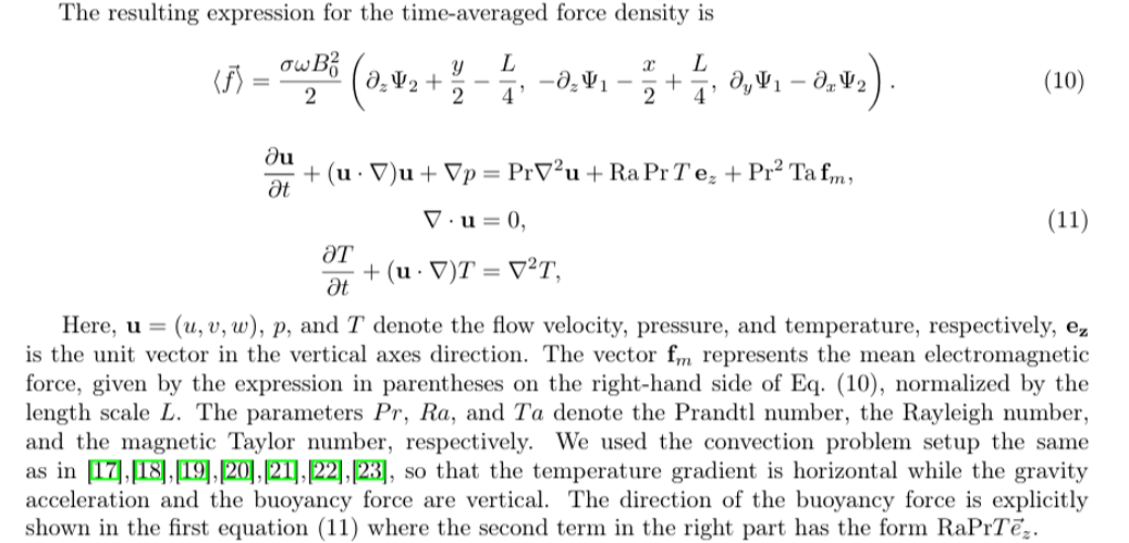
First, we compute the electromagnetic force
In[]:=
{Lx,Ly,Lz}={1,1,1};XYZgrid[dom_List,pts_List]:=MapThread[N@Range[Sequence@@#1,Abs[Subtract@@#1]/#2]&,{dom,pts-1}];Attributes[MakeVariables]={Listable};MakeVariables[var_,n_]:=Table[Unique[var],{n}];FDMat[deriv_,xygrid_,difforder_]:=Map[NDSolve`FiniteDifferenceDerivative[#,xygrid,"DifferenceOrder"->difforder]["DifferentiationMatrix"]&,deriv]{domain,pts,difforder}={{{0,Lx},{0,Ly},{0,Lz}},{11,11,11},4};xyzgrid=XYZgrid[domain,pts];{nx,ny,nz}=Map[Length,xyzgrid];{dx,dy,dz,dx2,dy2,dz2}=FDMat[{{1,0,0},{0,1,0},{0,0,1},{2,0,0},{0,2,0},{0,0,2}},xyzgrid,difforder];sgrid=Flatten[Outer[List,Sequence@@xyzgrid],2];{left1,right1,bot,top,left,right}={DeleteCases[Table[If[sgrid[[i,2]]==domain[[2,1]],i],{i,Length[sgrid]}],Null],DeleteCases[Table[If[sgrid[[i,2]]==domain[[2,2]],i],{i,Length[sgrid]}],Null],DeleteCases[Table[If[sgrid[[i,3]]==domain[[3,1]],i],{i,Length[sgrid]}],Null],DeleteCases[Table[If[sgrid[[i,3]]==domain[[3,2]],i],{i,Length[sgrid]}],Null],DeleteCases[Table[If[sgrid[[i,1]]==domain[[1,1]],i],{i,Length[sgrid]}],Null],DeleteCases[Table[If[sgrid[[i,1]]==domain[[1,2]],i],{i,Length[sgrid]}],Null]};boundaries=Join[top,bot,right1,left1,right,left];{uvar1,vvar1}=MakeVariables[{uu,vv},nxnynz];eqnu=(dx2+dy2+dz2).uvar1;eqnv=(dx2+dy2+dz2).vvar1;eqnu[[left]]=(dx.uvar1-sgrid[[All,3]]+.5)[[left]];eqnu[[right]]=(dx.uvar1-sgrid[[All,3]]+.5)[[right]];eqnu[[left1]]=(dy.uvar1)[[left1]];eqnu[[right1]]=(dy.uvar1)[[right1]];eqnu[[top]]=(dz.uvar1+sgrid[[All,1]]-.5)[[top]];eqnu[[bot]]=(dz.uvar1+sgrid[[All,1]]-.5)[[bot]];eqnv[[left1]]=(dy.vvar1-sgrid[[All,3]]+.5)[[left1]];eqnv[[right1]]=(dy.vvar1-sgrid[[All,3]]+.5)[[right1]];eqnv[[left]]=(dx.vvar1)[[left]];eqnv[[right]]=(dx.vvar1)[[right]];eqnv[[top]]=(dz.vvar1+sgrid[[All,2]]-.5)[[top]];eqnv[[bot]]=(dz.vvar1+sgrid[[All,2]]-.5)[[bot]];eqn=Join[eqnu,eqnv];var=Join[uvar1,vvar1];{vec,mat}=CoefficientArrays[eqn,var];sol=LinearSolve[mat,-vec];{U,V}=Partition[sol,Length[sgrid]];{fx,fy,fz}={1/8(-1+2sgrid[[All,2]]+4dz.V),1/8(1-2sgrid[[All,1]]-4dz.U),1/2(dy.U-dx.V)};
Visualization
{Fx,Fy,Fz}=Map[Interpolation@Join[sgrid,Transpose@List@#,2]&,Partition[Join[fx,fy,fz],Length[sgrid]]];VectorPlot3D2{Fx[x,y,z],Fy[x,y,z],Fz[x,y,z]},{x,0,1},{y,0,1},{z,0,1},
Out[]=
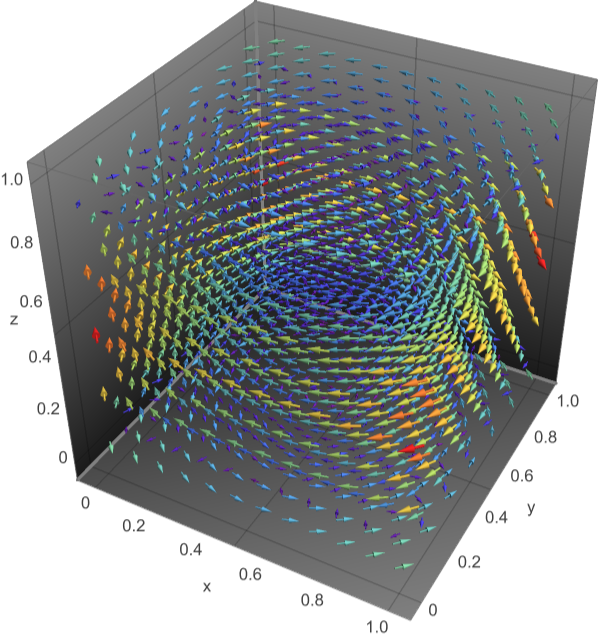
Next, we compute convection flow
In[]:=
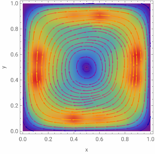
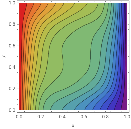
sols0[t0_,Pr_,Ra_,Ta_]:=Module[{tmax,dt=0.01},tmax=Round[t0/dt];boundaries=Join[top,bot,right1,left1,right,left];{uvar1,vvar1,wvar1,tvar1,pvar1}=MakeVariables[{uu,vv,ww,tt,pp},nxnynz];{uvar0,vvar0,wvar0,tvar0,pvar0}=Table[ConstantArray[0,{nxnynz,tmax}],{5}];Do[{uvar,vvar,wvar,tvar,pvar}={uvar0[[All,i]],vvar0[[All,i]],wvar0[[All,i]],tvar0[[All,i]],pvar0[[All,i]]};{uvar2,vvar2,tvar2,wvar2}={uvar0[[All,i-1]],vvar0[[All,i-1]],tvar0[[All,i-1]],wvar0[[All,i-1]]};cdu=(3uvar1-4uvar+uvar2)/(2dt);cdv=(3vvar1-4vvar+vvar2)/(2dt);cdw=(3wvar1-4wvar+wvar2)/(2dt);cdt=(3tvar1-4tvar+tvar2)/(2dt);eqnu=cdu+uvar(dx.uvar1)+vvar(dy.uvar1)+wvar(dz.uvar1)-Pr(dx2+dy2+dz2).uvar1+dx.pvar1-2TaPr^2fx;eqnv=cdv+uvar(dx.vvar1)+vvar(dy.vvar1)+wvar(dz.vvar1)-Pr(dx2+dy2+dz2).vvar1+dy.pvar1-2TaPr^2fy;eqnt=cdt+uvar(dx.tvar1)+vvar(dy.tvar1)+wvar(dz.tvar1)-(dx2+dy2+dz2).tvar1;eqnw=cdw+uvar(dx.wvar1)+vvar(dy.wvar1)+wvar(dz.wvar1)-Pr(dx2+dy2+dz2).wvar1+dz.pvar1-RaPrtvar1-2TaPr^2fz;eqnp=dx.uvar1+dy.vvar1+dz.wvar1;eqnu[[boundaries]]=uvar1[[boundaries]];eqnv[[boundaries]]=vvar1[[boundaries]];eqnw[[boundaries]]=wvar1[[boundaries]];eqnt[[left1]]=(dy.tvar1)[[left1]];eqnt[[right1]]=(dy.tvar1)[[right1]];eqnt[[left]]=tvar1[[left]]-1;eqnt[[right]]=tvar1[[right]];eqnt[[bot]]=(dz.tvar1)[[bot]];eqnt[[top]]=(dz.tvar1)[[top]];eqn=Join[eqnu,eqnv,eqnw,eqnt,eqnp];var=Join[uvar1,vvar1,wvar1,tvar1,pvar1];{vec,mat}=CoefficientArrays[eqn,var];sols=LinearSolve[mat,-vec];{uvar0[[All,i+1]],vvar0[[All,i+1]],wvar0[[All,i+1]],tvar0[[All,i+1]],pvar0[[All,i+1]]}=Partition[sols,Length[sgrid]];,{i,2,tmax-1}];]Pr0=0.065;tm=5;sols0[tm,Pr0,10^4,10^5]//AbsoluteTiming
Out[]=
{203.148,Null}
It takes 5-10 min depending on CPU. Visualization:
In[]:=
{u,v,w,T,p}=Map[Interpolation@Join[sgrid,Transpose@List@#,2]&,Partition[sols,Length[sgrid]]];
Horizontal flow and Temperature
In[]:=
ShowDensityPlotNorm[{u[x,y,.5],v[x,y,.5]}],{x,0,1},{y,0,1},,StreamPlot[{u[x,y,.5],v[x,y,.5]},{x,0,1},{y,0,1}],ContourPlotT[x,y,.5],{x,0,1},{y,0,1},
Out[]=
,

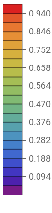
Vertical flow and temperature
With this code we can simulate transition to turbulence as it described in our paper. For example, using solution from above we can visualize the chaotic dynamics
Although we’ve tested this code very well, I still have questions concerning computational time and FDM. Can we solve this problem using FEM? Maybe we should use low-level programming the same as we used for FDM?
CITE THIS NOTEBOOK
CITE THIS NOTEBOOK
Numerical simulation and nonlinear dynamics in rotating magnetoconvection: chaos, attractors, and stability transitions
by Mutaz Mohammad and Alexander Trounev
Wolfram Community, STAFF PICKS, January 6, 2026
https://community.wolfram.com/groups/-/m/t/3602194
by Mutaz Mohammad and Alexander Trounev
Wolfram Community, STAFF PICKS, January 6, 2026
https://community.wolfram.com/groups/-/m/t/3602194