In[]:=
ClearAll["`*"]
In[]:=
GL[α_,λ_,m_,s_]:=;
λ
s
a+b+c
m
s
α
s
In[]:=
gnum[α_,λ_,m_,t_]:=Module[{f,s,R},f[s_]:=GL[α,λ,m,s];R=InverseLaplaceTransform[f[s],s,t,Method->"Talbot"];R];
In[]:=
ganal[α_,λ_,m_,t_]:=Module{p,q,n,P,r,g},p=Numerator[Rationalize[α]];q=Denominator[Rationalize[α]];n=Max[mq,p];P[z_]:=a+b+c;r=z/.Solve[P[z]==0,z];g=;g//Chop;
mq
z
p
z
1/q-1-λ
t
n
∑
k=1
MittagLefflerE[1q,1q-λ,r[[k]]]
1/q
t
P'[r[[k]]]
In[]:=
ganalSum[α_,λ_,m_,t_,M_]:=Sum**,{n,0,M},{r,0,M}//N;
Pochhammer[1,n+r]
Gamma[α-λ]Pochhammer[α-λ,rα+n(-m+α)]
-1+α-λ
t
r
-
c
α
t
b
n
-
a
-m+α
t
b
b
1
r!n!
In[]:=
a=2.1;b=1.3;c=1.4;α=10/3;λ=1.3;m=2;t=3.4;
In[]:=
gnum[α,λ,m,t]
Out[]=
-0.508039
In[]:=
ganal[α,λ,m,t]
Out[]=
-0.508039
In[]:=
ganalSum[α,λ,m,t,20]
Out[]=
-0.508039
In[]:=
ClearAll["`*"]
In[]:=
HoldFormInverseLaplaceTransform,s,t==Sum**,{n,0,Infinity},{r,0,Infinity}==*SrivastavaDaoustF[α-λ,1,-ct^α/b,-at^(α-m)/b]//TraditionalForm
λ
s
a+b+c
m
s
α
s
Pochhammer[1,n+r]
Gamma[α-λ]Pochhammer[α-λ,rα+n(-m+α)]
-1+α-λ
t
r
-
c
α
t
b
n
-
a
-m+α
t
b
b
1
r!n!
-1+α-λ
t
bGamma[α-λ]
Out[]//TraditionalForm=
-1
ℒ
s
λ
s
a+b+c
m
s
α
s
∞
∑
n=0
∞
∑
r=0
(1)
n+r
-1+α-λ
t
r
-
c
α
t
b
n
-
a
-m+α
t
b
Γ(α-λ)b(r!n!)
(α-λ)
rα+n(-m+α)
-1+α-λ
t
c
α
t
b
a
α-m
t
b
bΓ(α-λ)
(*--------------------------------------------------------------------------------------*)
For: y[0]=0, y’[0]=0 and f[t]=1+;
t
In[]:=
ClearAll["`*"]
In[]:=
S=LaplaceTransform[y[t],t,s]/.Solve[LaplaceTransform[ay''[t]+b*CaputoD[y[t],{t,3/2}]+cy[t]1+
t
,t,s]/.y[0]->0/.y'[0]->0,LaplaceTransform[y[t],t,s]][[1]]Out[]=
0.886227
3/2
s
1.
s
3.4+2.6+1.3
3/2
s
2
s
In[]:=
a=1.3;b=2.6;c=3.4;
In[]:=
G=InverseLaplaceTransform[S,s,t]
Out[]=
0.020050414.6689+(1.52664+3.72319)+(0.578268+0.802817)Erfc[(-0.578268-0.802817)]+(1.52664-3.72319)+(0.578268-0.802817)Erfc[(-0.578268+0.802817)]-(1.52664-0.713078)-(1.57827-0.425215)Erfc[(1.57827-0.425215)]-(1.52664+0.713078)-(1.57827+0.425215)Erfc[(1.57827+0.425215)]+0.022624413.-(2.10623-3.37861)+(0.578268+0.802817)Erfc[(-0.578268-0.802817)]-(2.10623+3.37861)+(0.578268-0.802817)Erfc[(-0.578268+0.802817)]+(2.10623-1.77458)-(1.57827-0.425215)Erfc[(1.57827-0.425215)]+(2.10623+1.77458)-(1.57827+0.425215)Erfc[(1.57827+0.425215)]
0.5
t
0.56419
0.5
t
(-0.310121+0.928486)t
2.71828
0.5
t
0.56419
0.5
t
(-0.310121-0.928486)t
2.71828
0.5
t
0.56419
0.5
t
(2.31012-1.34221)t
2.71828
0.5
t
0.56419
0.5
t
(2.31012+1.34221)t
2.71828
0.5
t
0.56419
0.5
t
(-0.310121+0.928486)t
2.71828
0.5
t
0.56419
0.5
t
(-0.310121-0.928486)t
2.71828
0.5
t
0.56419
0.5
t
(2.31012-1.34221)t
2.71828
0.5
t
0.56419
0.5
t
(2.31012+1.34221)t
2.71828
0.5
t
In[]:=
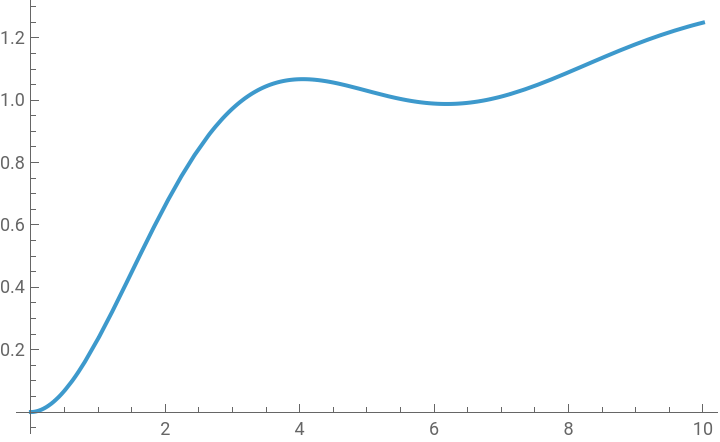
Plot[G,{t,0,10}]
Out[]=