The 3-colored distributed consensus problem
by Ryan Lau
BSc Natural Sciences (Physics & Physical Chemistry), University College London (UCL)
by Ryan Lau
BSc Natural Sciences (Physics & Physical Chemistry), University College London (UCL)
Abstract: Consider a collection of cells with a certain fraction of 3 distinct colours. There is some rule, of which when applied to the system, will turn all the cells to the majority colour when that fraction of the colours exceeds a certain threshold, reaching global consensus. The system will also exhibit indeterminate states when there are equal weights of colors. A general majority rule has been hypothesised and studied using grid cellular automata in cases of 2 and 3 colors. Some other rules are suggested, but their analysis is left for future studies. This report concludes with some criticism and possible future works.
Introduction
Introduction
The Idea
The Idea
The problem of distributed consensus has been well studied in the 2 colored case [1]. However, the existing literature is insufficient in solving for the problem of the 3-colored case. In this report, we will study this problem specifically on grid cellular automata. It is expected that the studies which will be conducted on the 3-colored case will provide some insight on how cellular automata links to certain properties in physical systems.
The problem
The problem
In this report, we will discuss some of the rules which perform on 3 colors, red, yellow and blue in 1-dimension (1D). The rules will be analogous to the majority function, similar to the GKL rule which will be discussed in future sections. The cells cannot decide which cell color is the majority, hence there will be indeterminate states of red yellow and blue. It is expected that the rule will provide us a “triple point” behaviour, where the cells cannot determine which color is the majority. The idea is studied via hypothesizing a general majority rule, and applying it to 2-colored and 3-colored system, with comparisons of their behaviours being made. Some other rules will also be suggested, but will be analysed in future works.
The Majority Function
The Majority Function
The main idea of the majority function or rule is that it returns the majority color of some neighbouring cells. The sections below will have some more concrete examples.
The GKL rule
The GKL rule
The Gacs-Kurdyumov-Levin (GKL) rule, or the “radius 3” rule operating on size-7 neighborhoods [1] provides us with a 1D deterministic cellular automaton rule that would lead to global consensus. Consider an initial system, Sys1, with a random arrangement of red cells with fraction p = 0.6. The rest will be yellow cells. The GKL rule as described by the following in the Wolfram Language is given as:
{l3_, _, l1_, c_, r1_, _, r3_} :> If[If[c == 0, r1 + r3, l1 + l3] + c >= 2, 1, 0]
We then apply it to the initial system Sys1:
In[]:=
Labeled[BlockRandom[SeedRandom[567];ArrayPlot[CellularAutomaton[{FromDigits[Tuples[{1,0},7]/.{l3_,_,l1_,c_,r1_,_,r3_}:>If[If[c==0,r1+r3,l1+l3]+c>=2,1,0],2],2,3},RandomChoice[{.6,.4}->{1,0},300],60],ColorRules->{0->Hue[0.15,0.72,1],1->Hue[0.98,1,0.8200000000000001]},Frame->False,ImageSize->Large]],"Fig 1: GKL rule when p = 0.6"]
Out[]=
Fig 1: GKL rule when p = 0.6 |

We can also consider another initial system, Sys2, with p = 0.4, and applying the same rule on it:
In[]:=
Labeled[BlockRandom[SeedRandom[569];ArrayPlot[CellularAutomaton[{FromDigits[Tuples[{1,0},7]/.{l3_,_,l1_,c_,r1_,_,r3_}:>If[If[c==0,r1+r3,l1+l3]+c>=2,1,0],2],2,3},RandomChoice[{.4,.6}->{1,0},300],60],ColorRules->{0->Hue[0.15,0.72,1],1->Hue[0.98,1,0.8200000000000001]},Frame->False,ImageSize->Large]],"Fig 2: GKL rule when p = 0.4"]
Out[]=
Fig 2: GKL rule when p = 0.4 |
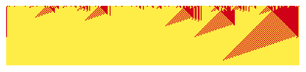
Both cases successfully reaches to a “global consensus”. The plot below shows how the colors of the grids change with time for different initial systems, or different values of p:
In[]:=
data=ParallelTable[If[p==.5,Nothing,MeanAround/@Transpose[Table[Mean/@CellularAutomaton[{FromDigits[Tuples[{1,0},7]/.{l3_,_,l1_,c_,r1_,_,r3_}:>If[If[c==0,r1+r3,l1+l3]+c>=2,1,0],2],2,3},RandomChoice[{p,1-p}->{1,0},5000],200],200]]],{p,.3,.7,.05}];Labeled[ListLinePlot[MapThread[Callout[#1,Row[{Style["p",Italic],"=",#2},ImageSize->Large]]&,{data,Cases[Range[.3,.7,.05],Except[0.5]]}]],"Fig 3: Plot of color tendencies against the number of steps for different values of p"]
Out[]=
Fig 1: GKL rule when p = 0.6 |

The y-axis shows the color tendencies (0 for yellow, 1 for red), and the x-axis shows the number of steps performed. The plot above shows properties which are similar to a phase transition [2]. For p < 0.5, the cells will be all yellow; for p > 0.5, the cells will be all red. However at p = 0.5, the cellular automaton is “indecisive”, hence generating the following nested pattern:
In[]:=
Labeled[BlockRandom[SeedRandom[24425];ArrayPlot[CellularAutomaton[{FromDigits[Tuples[{1,0},7]/.{l3_,_,l1_,c_,r1_,_,r3_}:>If[If[c==0,r1+r3,l1+l3]+c>=2,1,0],2],2,3},RandomChoice[{.5,.5}->{1,0},1000],500],ColorRules->{0->Hue[0.15,0.72,1],1->Hue[0.98,1,0.8200000000000001]},Frame->False,ImageSizeLarge]],"Fig 4: GKL rule when p = 0.5"]
Out[]=
Fig 4: GKL rule when p = 0.5 |

The image above shows us a “critical phenomenon” [3], much like the critical point we see in properties of matter, where the matter itself is indistinguishably in a gas and liquid state at some definite temperature and pressure.
The image above shows us a “critical phenomenon” [3], much like the critical point we see in properties of matter, where the matter itself is indistinguishably in a gas and liquid state at some definite temperature and pressure.
Rule 184
Rule 184
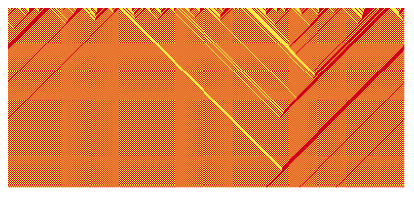
There are certain rules which gives us similar behaviour as discussed. For example, the rule 184 [4] when p = 0.5, with nested patterns of red and yellow stripes moving left and right :
In[]:=
Labeled[BlockRandom[SeedRandom[567];ArrayPlot[CellularAutomaton[184,RandomChoice[{1,0},400],180],ColorRules->{0->Hue[0.15,0.72,1],1->Hue[0.98,1,0.8200000000000001]},Frame->False,ImageSizeLarge]],"Fig 5: Rule 184 when p = 0.5"]
Out[]=
Fig 5: Rule 184 when p = 0.5 |
The Rules for the 3-Colored Problem
The Rules for the 3-Colored Problem
Method
Method
For this particular problem, there are too many rules which one might investigate. Conducting an exhaustive search will be practically unfeasible as it is computationally too expensive. Better heuristics should be developed to perform such searches. Therefore, we will first construct an analog of the GKL via trial and error, together with some random searches within a rules, using the CellularAutomaton function. We will expect the system to have some phase transition properties for different weights of the 3 colors.
Translation from 2-colored to 3-colored rules
Translation from 2-colored to 3-colored rules
One cannot apply a 2-colored rule to a 3-colored rule in cellular automata. As given in the documentation [5], the 1D general RuleNumber, n, is specified by the following:
n=
2r+1
k
k
(
1
)where k is the number of colors, and r the number of nearest neighbours. In our case there will be rules that are applicable to 3 colors, with varying r.
2r+1
3
3
Analog of the Majority Rule
Analog of the Majority Rule
The main goal of the majority rule is to let it decide on which color has the highest fraction after a certain number of steps. Here we can hypothesise a general majority rule as the following:
neighbors:{l3_,b3_,l1_,c_,r1_,b1_,r3_}:>First @ Commonest[neighbors]
Let us name the rule above Maj7. It operates on size-7 neighborhoods, and has a similar form as the GKL rule above. The overall rule number is given by the following:
FromDigits[Tuples[{1,0},7]/. neighbors:{l3_,b3_,l1_,c_,r1_,b1_,r3_}:>First @ Commonest[neighbors],k]
The k here indicates the number of colors in the system again. Let us see what it does on a two colored system, and have a plot to analyse what it gives us when p > 0.5 or p < 0.5:
In[]:=
Manipulate[ArrayPlot[CellularAutomaton[{FromDigits[Tuples[{1,0},7]/.neighbors:{l3_,b3_,l1_,c_,r1_,b1_,r3_}:>First@Commonest[neighbors],2],2,3},SeedRandom[seed];Normal[SparseArray[Thread[RandomSample[Range[400],Round[d400]]->1],400]],50,400],ImageSize->{500,369},PlotRange->{{0,w},{0,w}},PlotLabel->Text[Style["Fraction of red cell: "<>ToString[d],"Output",Bold]],ColorRules{0->Yellow,1->Red}],{{seed,1234,"Initial seeds "},1000,1500,1},{{d,0.5,"Fraction of red cell "},0.002,1},Delimiter,{{w,150,"zoom"},20,250,1}]
Out[]=


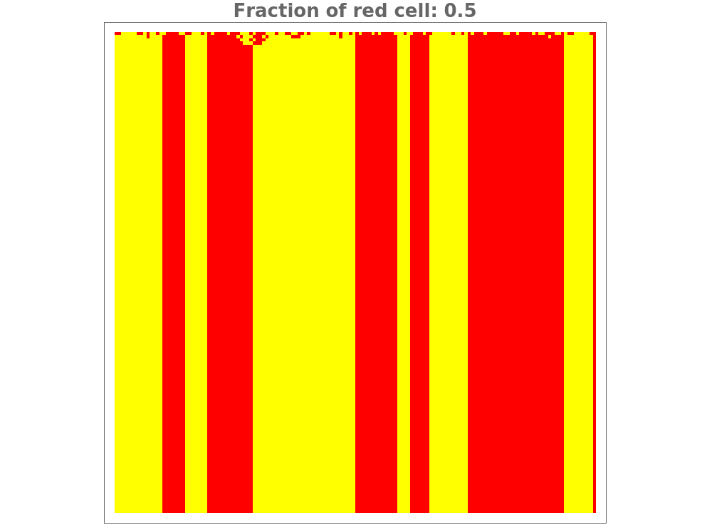
As we can see from Fig 6, there is a change of behaviour at p = 0.5, which are very similar to Fig 3. The difference is that the Maj7 rule does not help the system reach global consensus, only local consensus, unlike the GKL rule. We can then conclude the hypothesised rule does give some “phase transition” property when crossing
p = 0.5 .
From now onwards, let us label 0 as Yellow, 1 as Red and 2 as Blue for consistency throughout the code and notebook. Let us then look at what the Maj7 rule does with 3 colors:
p = 0.5 .
From now onwards, let us label 0 as Yellow, 1 as Red and 2 as Blue for consistency throughout the code and notebook. Let us then look at what the Maj7 rule does with 3 colors:
Plotting a line graph like Fig 6 is not so easy for the 3-colored case. As there are 3 colors, which the weights have to add up to one, and the three colors have to be plot against the number of steps, one would need to plot a 4D graph to fully describe the system. To simplify the problem, the blue color is chosen to be fixed to have fractions of 0.3 and 0.5, and we then vary colors yellow and red, and use ListLinePlot3D to plot a 3D analog of Fig 6 to see whether the rule also gives us some phase transition properties:
Conveniently, the red and yellow surfaces represents the colors red and yellow. The color tendency label is same as the color rules discussed before. Let us take Fig 8a for example. In the regime of low proportion of red colored cells or high proportion of yellow colored cells, the red colored cells will gradually turn into yellow colored cells, indicated by the decreasing color tendency towards the color yellow; The yellow colored cells will remain yellow, indicated by the unchanging gradient. The same applies to the opposite regime discussed. There exists a special point when two surfaces cross over each other (Color Proportion = 0.3 for Fig 8a ; Color Proportion = 0.5 for Fig 8b), which is when red and yellow have the same fraction. The crossing over in Fig 8a shows that the system cannot determine its majority color, shown by the unchanging gradient of the surface, as the 3 colors all are in equal weights. The crossing over in Fig 8b is different. While red and yellow have the same fraction, the majority color is blue, thus both red and yellow tends towards 0.5 after some steps. The rule therefore can determine the majority color successfully, but cannot reach global consensus. Although we can see the behaviours of the states, it is quite hard to interpret whether there are phase transition properties from above. To solve this problem future works, a plot can be made with fixing a step, but with varying weights of the 3 colors to get a bigger picture of the system and the majority rule itself.
I would also like to share some trial rules which gave some other interesting results:
Some other Rules via Random Searches
Some other Rules via Random Searches
According to equation (1), there are too many rules for the 3-colored system. Performing an exhaustive search of all the possible rules will be computationally too expensive. Alternatively, one can try to search the rule which leads to some indeterminate state and global consensus through trial and error. The systems below have equal proportions of yellow and red, and some randomly chosen rules are applied (you will see the rule numbers in the code):
Concluding remarks
Concluding remarks
General Criticism
General Criticism
The Maj7 rule above works for the 2-colored case. It shows a phase transition property, but cannot achieve global consensus. It is also not sure whether it works for the 3-colored one, as it reaches some sort of a local consensus, but not a global one. The 3D plot above does not show clearly whether the rule gives us phase transition properties or not. It is suggested that these rules should be built upon and modified, then studied using plots suggested in previous sections. It is natural to continue to study these systems in the future using grid cellular automata by adding and experimenting on different cases and condition, whilst linking it to physical systems.
Future Extensions
Future Extensions
Adding noise
Adding noise
One can add some “noise” in the system and study its properties, which has been done for the 2-colored case [1]. In the low noise regime, the GKL can still achieve consensus, while when some greater noise is present, the consensus is lost. The problem converts from an ordinary cellular automaton into a probabilistic one. If a more detailed graph describing the GKL rule is plotted, the result will be a conventional phase diagram as shown below. The same can be done in the 3-colored case.
“Derivation” of Rules
“Derivation” of Rules
The question of how to come up with these rules is a big question in this project. It will be simpler to systematically build up a rule which exhibits phase transition properties and helps the system to reach global consensus. Some function which returns the property of the rules may also be useful, such as RulePlot.
Beyond 1D
Beyond 1D
We have only discussed the 1D case. The model can be extended to the 2D and 3D cases in the future. The 2 colored case has been done in 2D and 3D. One needs to extend the rule parameters to more than 1D and will require totalistic rules, instead of rule numbers for the 1D case.
Linking to Physical Systems
Linking to Physical Systems
Following up on 2D cellular automaton, much has been done to use these models to describe fluid flow [6] and 2D spin chains, such as the Ising model [7], rather than using mathematical equations. The Ising model can be seen as a square lattice of electrons with their intrinsic angular momentum, or “spins” pointing up or down. Such models also give us some ideas on the origins of discreteness. It is believed that by studying these systems, more insight will arise and we may utilise it to explain other physical systems. For example, besides conventional symmetry breaking of conventional phases of matter, topological phase transitions as demonstrated by the Haldane spin chain [8] can be explained and understood via studying cellular automaton. A linkage to the renormalization group [9], which describes changing systems, will also be useful.
Generalisation to N-Colored Systems
Generalisation to N-Colored Systems
Although the work has been done for the 3-colored system, one may be able to generalise such rules into systems of more than 3-colors. The transformation rule from 2 colors to 3 colors has been done above. The code written can be generalised to convert any rules of a number of colored to another one, which will be helpful to include in the resource function for easier translations. Here is a preliminary demonstration of a 4-colored case, by adjusting the parameter k and adding the color black. Note that the 4 colors have equal proportions in this case:
Conclusion
Conclusion
This project raises more questions than it has answered. It is hoped that this work will be modified and built upon in the future to study similar systems and ultimately be used to some physical phenomena. In conclusion, we have come up with a hypothesised rule, the Maj7 Rule , which in the 2-color regime, exhibits phase transition behaviours and reaches local consensus. When applied to the 3-color system, the rule successfully determines the majority color but not achieving global consensus. It is unclear the Maj7 rule gives phase transition or triple point properties, which can be solved in future works. Lastly, some ideas of future extensions are given.
Acknowledgments
Acknowledgments
I would like to thank Dr. Stephen Wolfram for defining this project for me; my mentors, Hatem and Mano for giving my insights to conduct the project; Nik, Jesse, Silvia, Carlos and other TAs for helping me to debug and fix my code; all the lecturers and speakers for giving amazing and informative talks; all other staff members and students which made this unforgettable experience happen.
I would like to thank Dr. Stephen Wolfram for defining this project for me; my mentors, Hatem and Mano for giving my insights to conduct the project; Nik, Jesse, Silvia, Carlos and other TAs for helping me to debug and fix my code; all the lecturers and speakers for giving amazing and informative talks; all other staff members and students which made this unforgettable experience happen.
References
References
◼
[8] F.D.M. Haldane, Phys. Rev. Lett. 50, 1153 (1983)