Abstract
Abstract
eBird is a birding service run by Cornell University. It allows its users to submit data about their bird sightings, and stores them to be viewed for later. More importantly, it stores this data in a large database of bird sightings. Much of this data is uploaded to the Global Biodiversity Information Facility, or GBIF, a worldwide repository with data for all species known on Earth. Its bird data is used here to generate graphs of where birds coexist, for a specified region and time.
Introduction
Introduction
Originally, when starting this project, I had no knowledge of the GBIF. I had been working with eBird's EBD, or eBird Basic Dataset, a small set of example data. Most of the code was built using that, but it thankfully transferred neatly to the GBIF data. Here, I'll define some variables, as well as import the data.
The location and time span that will be used in this talk are:
January to July , near Barnegat Light, New Jersey, United States
(It’s relatively near to me and recommended for study by my father, resident birder of my house.)
January
st
1
st
1
(It’s relatively near to me and recommended for study by my father, resident birder of my house.)
Here, we define the position of Barnegat Light and define the time range:
In[]:=
GeoGraphics[GeoBoundsRegion[{{minLatitude,maxLatitude},{minLongitude,maxLongitude}}]]
Out[]=
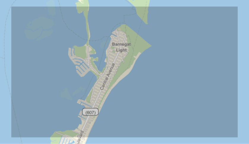
In[]:=
minLatitude=39.73;maxLatitude=39.77;minLongitude=-74.15;maxLongitude=-74.06;minDate="2020-01-01";maxDate="2020-07-01";gridUnit=1/360;
Here we have bird data for our region:
In[]:=
baseURL="https://api.gbif.org/v1/occurrence/search";gbifURL=StringReplace[URLBuild[baseURL,{"decimalLatitude"ToString@minLatitude<>","<>ToString@maxLatitude,"decimalLongitude"ToString@minLongitude<>","<>ToString@maxLongitude,"eventDate"minDate<>","<>maxDate,"taxonKey"212}],"%2C"","];gbifData=URLExecute[HTTPRequest[gbifURL,<|"Method""GET"|>]];dataRows=Association/@Association[gbifData]["results"];dataRows〚1〛//Keys(*Wehavequiteafewproperties*)
Out[]=
{key,datasetKey,publishingOrgKey,installationKey,publishingCountry,protocol,lastCrawled,lastParsed,crawlId,extensions,basisOfRecord,taxonKey,kingdomKey,phylumKey,classKey,orderKey,familyKey,genusKey,speciesKey,acceptedTaxonKey,scientificName,acceptedScientificName,kingdom,phylum,order,family,genus,species,genericName,specificEpithet,taxonRank,taxonomicStatus,dateIdentified,decimalLongitude,decimalLatitude,stateProvince,year,month,day,eventDate,issues,modified,lastInterpreted,references,license,identifiers,media,facts,relations,geodeticDatum,class,countryCode,recordedByIDs,identifiedByIDs,country,rightsHolder,identifier,http://unknown.org/nick,verbatimEventDate,datasetName,collectionCode,verbatimLocality,gbifID,occurrenceID,taxonID,catalogNumber,recordedBy,http://unknown.org/occurrenceDetails,institutionCode,rights,eventTime,occurrenceRemarks,identifiedBy,identificationID}
What birds?
What birds?
One issue that originated while working with the EBD is that there are too many birds. Seriously. Not necessarily sightings, but there are so many different species! In the EBD (which was just around Montgomery, Alabama, US), there were 119 different species; plotting those in one graph becomes… problematic, to say the least. Thankfully, there aren't that many birds in the Barnegat Light region. Other variables are also defined in this stage related to the names of birds.
Here, we get the scientific as well as common names of the birds:
In[]:=
birdNames=dataRows〚All,"acceptedScientificName"〛//DeleteDuplicates;commonBirdName[bird_]:=Interpreter["Species"][StringRiffle[StringSplit[bird]〚;;2〛]]["Name"]birdCounts=CountsBy[dataRows,#["acceptedScientificName"]&];Grid[Join[{{"Scientific Name","Common Name","Count"}},Transpose@{birdNames,commonBirdName/@birdNames,Values@birdCounts}],FrameAll]
Out[]=
Scientific Name | Common Name | Count |
Histrionicus histrionicus (Linnaeus, 1758) | harlequin duck | 4 |
Gavia immer (Brunnich, 1764) | common loon | 2 |
Arenaria interpres (Linnaeus, 1758) | ruddy turnstone | 1 |
Larus smithsonianus Coues, 1862 | American herring gull | 3 |
Somateria mollissima dresseri Sharpe, 1871 | common eider | 1 |
Clangula hyemalis (Linnaeus, 1758) | oldsquaw | 1 |
Turdus migratorius migratorius | American robin | 1 |
Calidris maritima (Brunnich, 1764) | purple sandpiper | 1 |
Gavia stellata (Pontoppidan, 1763) | red-throated loon | 2 |
Melanitta nigra americana (Swainson, 1832) | common scoter | 2 |
Melanitta fusca deglandi (Bonaparte, 1850) | velvet scoter | 2 |
Bird Locations
Bird Locations
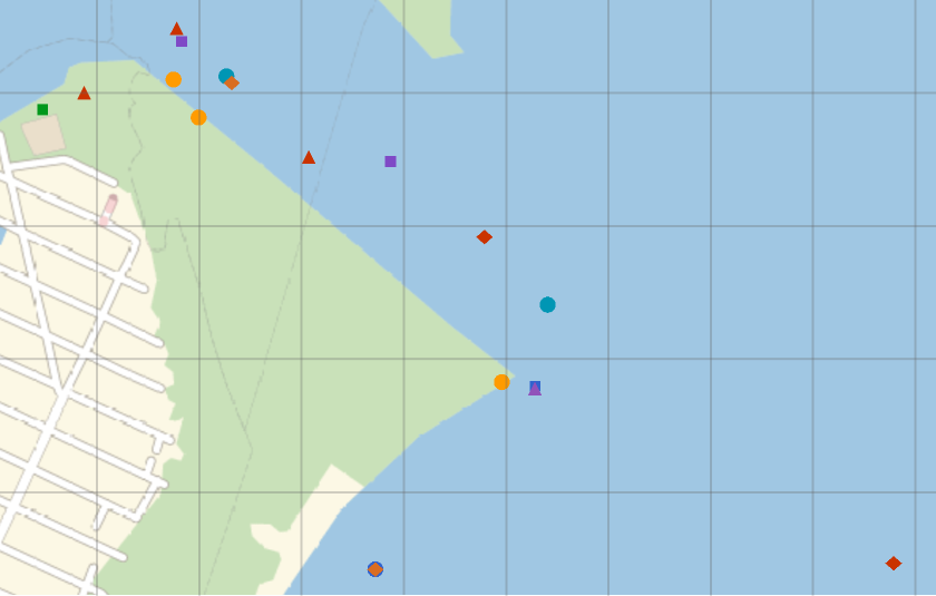
If we want to find out what birds coexist, we need to figure out where they exist in the first place. As with all sighting data, the GBIF data contains a field with the longitude and latitude, both represented as decimals. Plotting the birds' locations on a map is a helpful visual tool.
Plotting time! Each bird is plotted in a different style, as to differentiate between them:
In[]:=
GeoListPlot[Map[GeoPosition,Values[ToExpression/@GatherBy[dataRows,#["acceptedScientificName"]&]〚All,All,Key/@{"decimalLatitude","decimalLongitude"}〛],{2}],PlotLegendsPlaced[(dataRows〚All,Key["acceptedScientificName"]〛//DeleteDuplicates),Below],GeoGridLinesQuantity[gridUnit,"AngularDegrees"]]
Out[]=


Functions Galore
Functions Galore
(ok fine it's just four)
(ok fine it's just four)
In order to generate a graph, we need to define a few functions; in my code, I have four. They are as follows in the code below. You may wonder, "Why would you define all those functions?" Well, you see, these are used to figure out bounding squares for each bird, and finding things about those.
IndividualBirdRange: gets a range for a bird sighting
birdLocations: gets all locations for a single bird
GridSquares: gives birds proper squares on a grid defined by one variable, gridUnit
BirdSquares: GridSquares for a species
birdLocations: gets all locations for a single bird
GridSquares: gives birds proper squares on a grid defined by one variable, gridUnit
BirdSquares: GridSquares for a species
In[]:=
rangeDeviation=1/4;IndividualBirdRange[birdloc_]:=Module[{a=Floor[birdloc〚1〛,gridUnit],b=Ceiling[birdloc〚1〛,gridUnit],c=Floor[birdloc〚2〛,gridUnit],d=Ceiling[birdloc〚2〛,gridUnit],relLat=Mod[birdloc〚1〛,gridUnit],relLong=Mod[birdloc〚2〛,gridUnit]},{Which[relLat≥(1-rangeDeviation)gridUnit,{a,b+gridUnit},(rangeDeviation)gridUnit>relLat,{a-gridUnit,b},True,{a,b}],Which[relLong≥(1-rangeDeviation)gridUnit,{c,d+gridUnit},(rangeDeviation)gridUnit>relLong,{c-gridUnit,d},True,{c,d}]}]birdLocations[bird_]:=Values[ToExpression/@Select[dataRows,bird==#["acceptedScientificName"]&]〚All,Key/@{"decimalLatitude","decimalLongitude"}〛];GridSquares[{{a_,b_},{c_,d_}}]:=Flatten[Table[{{i,i+gridUnit},{j,j+gridUnit}},{i,a,b-gridUnit,gridUnit},{j,c,d-gridUnit,gridUnit}],1]BirdSquares[bird_]:=Flatten[GridSquares[IndividualBirdRange[#]]&/@birdLocations[bird],1]
Final Graph
Final Graph
We're finally ready to make the graph! Here, I define a few things:
(1) coexistence[], a function based on the previous section
(2) coexistenceThreshold, a bar for the coexistence of birds to be above
(3) The adjacency matrix for the graph, and more importantly, the graph!
(1) coexistence[], a function based on the previous section
(2) coexistenceThreshold, a bar for the coexistence of birds to be above
(3) The adjacency matrix for the graph, and more importantly, the graph!
The graph has edge thickness defined by the value of the coexistence function. This can be changed, if desired, in a personal copy of this notebook.
Future Work/Extensions
Future Work/Extensions
Even though we have some very pretty graphs, a lot can still be done with this project. Here are my ideas for extending the project:
◼
I want to have a lot more interactivity; sadly, Manipulate[] and similar functions wouldn't work here, but I want to make a form where the user can input many different specifications. I want to allow full control of the GBIF's API parameters for future progress.
◼
After posting the first draft of this essay, I was alerted to the existence of a resource function GBIFSearch. In all fairness, it was created one day before the first draft of the essay, but I would like to use that as to clean up the code.
◼
Due to an interesting fact of how the GBIF API works, one parameter (the taxonKey) can be changed to specify other kinds of species. I'm not too sure how to find a specific taxon key, but I would like to look into using this code for other species.
◼
While editing this computational essay, I realized that the coexistence function would probably make more sense to be distance-related; however, a simple redefinition of the coexistence function would suffice to do that. I tried to make as many parts of this code relatively easy to adjust; hence, the coexistence function/threshold, rangeDeviation, gridUnit… in future, I would like to try and make as many things this way as possible.
◼
Eventually, if it is possible, I want to have the graph plotted on a map of the region, with each vertex at the mean location for each species.
Acknowledgements
Acknowledgements
I would like to thank the directors of Wolfram Summer Camp 2020 for holding the camp;
Harshal Gajjar, for being my mentor and helping me with many coding troubles;
and last but not least, my father, Todd Gilbert, for reference on any facts/theories relating to birds.
Harshal Gajjar, for being my mentor and helping me with many coding troubles;
and last but not least, my father, Todd Gilbert, for reference on any facts/theories relating to birds.
References
References
◼
GBIF - The GBIF website, from which I found out how to get the data
◼
api.gbif.org/v1 - the GBIF API, from which I got the aforementioned data
◼
eBird - The eBird website, without which this project would not have been possible
Keywords
Keywords
◼
Graph Theory
◼
Birds
◼
eBird
◼
GBIF