Borda Count is a ranking voting system in which the voters rank the candidates instead of picking one candidate, effectively rewarding the candidate that is acceptable to the majority instead of one that is especially favored by some. However, Borda Count can be especially vulnerable to strategic voting—that is, voting not according to true preference but in order to manipulate the result in some way. This project tests the impact of strategies such as burying, compromising, and a mix of both on the final candidate elected, how happy people are with the candidate, and whether this candidate tends to be extreme or moderate.
Introduction
Introduction
The pursuit of a perfectly fair democratic election has existed for as long as humans have had to make collective decisions. Among the many voting systems that have been proposed, the Borda Count stands out for its theoretical ability to elect a candidate that is widely accepted instead of simply one that most people consider as their first choice. This voting method assigns a descending number of points to candidates based on their ranking on a voter’s ballot. For example, in an election with N candidates, the candidate ranked kth place receives N - k points.
However, this system may encourage voters to vote strategically rather than according to their true preferences. This project examines the impact of different types of strategic voting on the result of the election.
However, this system may encourage voters to vote strategically rather than according to their true preferences. This project examines the impact of different types of strategic voting on the result of the election.
Generating Voters and Candidates
Generating Voters and Candidates
Voters and candidates are represented by their political positions. These political positions are separated into their opinions on different policy issues (such as education) which I call issues, with a point on a 2D graph portraying the specific stance of the person on that issue. This 2D graph can be seen as a representation of the political compass, where the x-axis serves as the economic axis (Left and Right) and the y-axis serves as the Social Axis (Authoritarian and Libertarian); in this case, a position of {0.5,0.5} on the issue of education can be interpreted as meaning that the particular person believes in a more Authoritarian and Right governmental approach. Under this definition, a voter would favor a candidate more if their beliefs are closer in position to the candidate’s beliefs.
To simulate a more realistic distribution of opinions, each voter and candidate is given an overall ideological position generated through a bivariate normal distribution, so that more people tend to be more moderate. Then, their specific ideological positions for each issue are generated as another bivariate normal distribution centered on the overall ideological position. While everyone has an overall ideological tendency, their beliefs for each issue may vary somewhat.
To simulate a more realistic distribution of opinions, each voter and candidate is given an overall ideological position generated through a bivariate normal distribution, so that more people tend to be more moderate. Then, their specific ideological positions for each issue are generated as another bivariate normal distribution centered on the overall ideological position. While everyone has an overall ideological tendency, their beliefs for each issue may vary somewhat.
Generating Positions
Generating Positions
Generates a voter based on how many issues there are, and returns the voter’s standings on all of those issues:
In[]:=
biasedVoter[issues_]:=RandomVariate[BinormalDistribution[RandomVariate[BinormalDistribution[{0,0},{0.4,0.4},0]],{0.15,0.15},0],issues]
For example, one voter considering 5 issues could look like:
In[]:=
voterExample=biasedVoter[5]
Out[]=
{{-0.379877,-0.363977},{-0.249071,-0.256433},{-0.469066,-0.472834},{-0.31971,-0.341283},{-0.298351,-0.641436}}
Generates a group of these voters, each with their own overall ideological position and specific positions for each issue:
In[]:=
biasedGroupVoters[population_,issues_]:=Table[biasedVoter[issues],population]
For example, a group of 5 voters considering 5 issues could look like:
In[]:=
votersExample=biasedGroupVoters[5,5]
Out[]=
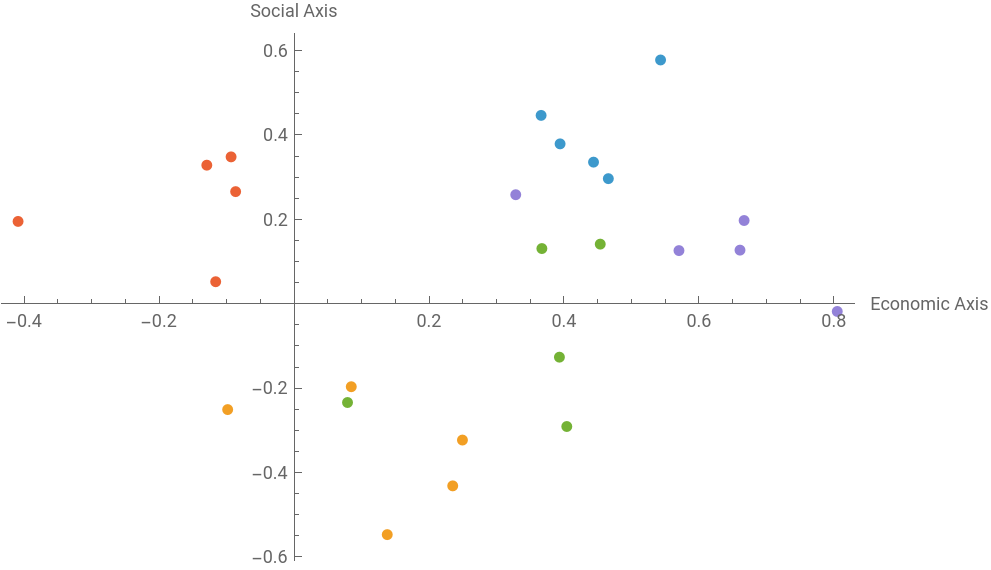
{{{0.443763,0.335608},{0.394205,0.378893},{0.543105,0.577681},{0.366086,0.446379},{0.465703,0.296493}},{{0.138087,-0.546987},{-0.0983959,-0.250703},{0.235109,-0.43145},{0.0847584,-0.196553},{0.249512,-0.322919}},{{0.453717,0.141311},{0.404147,-0.290813},{0.39322,-0.126497},{0.0792127,-0.233948},{0.36722,0.130854}},{{-0.408993,0.195147},{-0.12929,0.328419},{-0.0933347,0.348078},{-0.0865844,0.265744},{-0.11614,0.0522628}},{{0.804936,-0.018199},{0.666914,0.197298},{0.328497,0.258418},{0.570374,0.126012},{0.660813,0.127114}}}
Putting all of the positions on the same graph, with each color representing the different issue positions for the same voter:
In[]:=
ListPlot[votersExample,AxesLabel->{"Economic Axis","Social Axis"}]
Out[]=
Similarly, this function generates a candidate:
In[]:=
biasedCandidate[issues_]:=RandomVariate[BinormalDistribution[RandomVariate[BinormalDistribution[{0,0},{0.4,0.4},0]],{0.15,0.15},0],issues]
One candidate considering 5 issues could look like:
In[]:=
candidateExample=biasedCandidate[5]
Out[]=
{{-0.199935,0.0471094},{0.0141294,-0.386401},{-0.532028,-0.288161},{-0.500556,-0.189513},{0.00258767,-0.374324}}
Generates a group of these candidates, similar to the voters:
In[]:=
biasedGroupCandidates[population_,issues_]:=Table[biasedCandidate[issues],population]
A group of 3 candidates considering 5 issues could look like:
In[]:=
candidatesExample=biasedGroupCandidates[3,5]
Out[]=
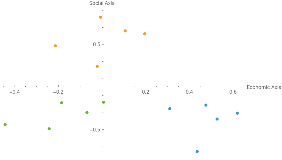
{{{0.619373,-0.306141},{0.526947,-0.375616},{0.435888,-0.757456},{0.310451,-0.254206},{0.475947,-0.211785}},{{-0.0220666,0.24428},{-0.00666223,0.820686},{-0.213402,0.484728},{0.106126,0.66019},{0.195745,0.626382}},{{-0.18443,-0.184623},{0.00705071,-0.177791},{-0.443583,-0.441},{-0.241931,-0.490679},{-0.0689147,-0.298098}}}
Putting all of the positions on the same graph, with each color representing the different issue positions for the same candidate:
In[]:=
ListPlot[candidatesExample,AxesLabel->{"Economic Axis","Social Axis"}]
Out[]=
Issue Weights
Issue Weights
Realistically, voters may not consider each issue equally. For example, someone who cares more about environmental conservation than national defense may rank higher a candidate that doesn’t align closely in their beliefs about national defense but aligns closely with their beliefs in environmental conservation, and rank lower a candidate that aligns closely in their beliefs about national defense but doesn’t align in their beliefs about environmental conservation. That is, one issue may be weighted more than another one. To incorporate this, I assigned random weights for each issue for each voter, such that a higher weight means that they take this issue more seriously and a lower weight means that the issue doesn’t really matter to them. If a voter has a higher sum of all of their weights, this voter cares more about politics in general.
Creates a list of how important each voter thinks each issue is:
In[]:=
issueWeights[issues_,voters_]:=Table[RandomReal[1,issues],{voters}]
For example, this could be the issueWeights of 5 voters and 5 issues:
In[]:=
issueWeightsExample=issueWeights[5,5]
Out[]=
{{0.696948,0.642269,0.609831,0.604017,0.404492},{0.494981,0.719124,0.707146,0.775807,0.804998},{0.130111,0.293884,0.604701,0.938602,0.851389},{0.953066,0.492701,0.943664,0.530257,0.080345},{0.433237,0.193281,0.355371,0.933494,0.218463}}
Finding and Evaluating the Winner
Finding and Evaluating the Winner
Creating Rankings
Creating Rankings
Under these assumptions, each voter ranks all of the candidates by how close each candidate is to them across all issues, taking into consideration how important they believe each issue is. For each voter-candidate pair, a vector of distances between the voter and the candidate is calculated, one distance for each issue. Then, the dot product is taken of this distance vector and the voter’s issue-Weight vector, created a weighted sum. This sum then determines the ranking that the voter gives the candidate.
Find all of the distances between each voter and each candidate, for each issue:
In[]:=
allDistances[candidates_,voters_]:=Table[EuclideanDistance[i[[k]],j[[k]]],{i,voters},{j,candidates},{k,Length[First[candidates]]}]
Using the voters and candidates that was generated earlier, all of the distances are:
In[]:=
allDistancesExample=allDistances[candidatesExample,votersExample]
Out[]=
{{{0.665343,0.766096,1.33944,0.70279,0.508382},{0.474698,0.596553,0.762197,0.336592,0.426268},{0.815639,0.678074,1.41819,1.11703,0.799597}},{{0.538185,0.637697,0.382874,0.23294,0.252238},{0.807311,1.07531,1.02007,0.857009,0.950823},{0.485103,0.1282,0.678759,0.439587,0.319392}},{{0.477133,0.149236,0.6324,0.232124,0.359476},{0.486798,1.18499,0.861154,0.894543,0.524359},{0.716564,0.412867,0.893953,0.41115,0.611729}},{{1.14404,0.962451,1.22568,0.654206,0.648297},{0.390034,0.507311,0.181905,0.439004,0.653365},{0.441196,0.524249,0.863317,0.772211,0.35353}},{{0.342555,0.589764,1.02153,0.46057,0.386041},{0.867657,0.917779,0.587257,0.707723,0.682318},{1.00327,0.75902,1.04177,1.01988,0.844576}}}
Creates the rankings that the voters give the candidates, based on the weighted sum of the distances using weights; a ranking of {2,3,1}, for example, means that candidate 2 is ranked first, candidate 3 is ranked second, and candidate 1 is ranked last/third:
In[]:=
biasedRankingsWithWeights[candidates_,voters_,weights_]:=Ordering/@Table[Table[weights[[voterIndex]].candidateIndex,{candidateIndex,Table[EuclideanDistance[voterPosition[[issues]],candidatePosition[[issues]]],{voterPosition,voters},{candidatePosition,candidates},{issues,Length[First[candidates]]}][[voterIndex]]}],{voterIndex,Length[weights]}]
Using the voters, candidates, and weights generated earlier, the rankings are:
In[]:=
rankingsExample=biasedRankingsWithWeights[candidatesExample,votersExample,issueWeightsExample]
Out[]=
{{2,1,3},{1,3,2},{1,3,2},{2,3,1},{1,2,3}}
Tallying the Rankings and Finding the Winner
Tallying the Rankings and Finding the Winner
After all of the rankings are found, they have to be tallied to find the winner. As defined before, a candidate ranked last place by a voter receives a score of 0 from that voter’s ranking, and a candidate ranked second to last receives a score of 1 from that voter’s ranking.
Associations are made between the candidates and the number of scores they are getting from this ranking; then, the scores are totaled, creating a bigger association with candidates and the total score they get:
In[]:=
rankingScores[rankings_]:=KeySort[Merge[AssociationThread[#->Reverse[Range[0,Length[rankings[[1]]]-1]]]&/@rankings,Total]]
Tallying all of the scores from the rankings generated before:
In[]:=
scoresExample=rankingScores[rankingsExample]
Out[]=
17,25,33
If there are no ties, a winner is chosen directly. If there are any ties, they go head-to-head against each other, where the person who is ranked above the other more times wins a point (if the head-to-head is again a tie, the candidate represented by the smaller number directly wins). Then, the candidate with the most amount of points wins (if this is a tie, the candidate represented by the smaller number wins). The goal is to try to find the best winner, even if there are multiple candidates tied.
Between two candidates, finds the candidate that was ranked before more times; if this is a tie, finds the candidate represented by the smaller number:
In[]:=
headToHeadWinner[rankings_,a_,b_]:=Which[Count[Table[Which[First@First@Position[i,a]<First@First@Position[i,b],a,True,b],{i,rankings}],a]>(Length[rankings]/2),a,Count[Table[Which[First@First@Position[i,a]<First@First@Position[i,b],a,True,b],{i,rankings}],a]<(Length[rankings]/2),b,True,First@TakeSmallest[{a,b},1]]
In this example, in the first and second ranking, 1 is ranked before 2, and in the final ranking, 2 is ranked before 1, making 1 the winner in a head-to-head comparison:
Finds the winner given a ranking, using the headToHead function if there is a tie:
Finding the winner from the rankings made before:
Evaluating the Winner
Evaluating the Winner
Important insights into the effectiveness of voting systems include how closely the chosen winner matches the voters’ beliefs and whether the winner is moderate or extreme.
Happiness
Happiness
The winner’s alignment with the positions of the voters is named Happiness, and it is calculated through the weighted sum of the distance between the candidate’s positions and all of the positions of the voters. Similar to creating rankings, this is found through the reciprocal of the weighted distance of the distances and issue weights of the voters, so that the higher the number, the happier people are with them. Therefore, a candidate that aligns with the voters on issues that are more important to them has a higher value of happiness than a candidate that aligns with the voters on issues that are less important. Similarly, a candidate that aligns with voters who care more about politics has a higher value of happiness than a candidate that aligns with the voters who care less about politics.
Finds the Happiness value that people are with the winner:
For example, looking at the winner from the election generated before:
Finds the Happiness value of all of the candidates:
Looking at all of the candidates from the election generated before:
Comparing the happiness of the all of the candidates:
If the winner is the candidate that has the highest Happiness value, then it is defined as the best winner.
Extremeness
Extremeness
The winner’s extremeness is found through comparing how far away from the origin it is to the other candidates. If the sum of the distances between the candidate position and the origin across different issues is greater than the average of the respective value across different candidates, that candidate is considered to be extreme.
Finds if the winning candidate is extreme:
Evaluating the extremeness of the winner elected from the election before:
Honest Borda Baseline
Honest Borda Baseline
Before testing how strategic voting influences the election, I first tested the results of an honest Borda. In the honest model, each voter ranks the candidates entirely according to weighted distance across issues.
To repeat this process, I created a function that runs an entire election and returns the results from that election.
To repeat this process, I created a function that runs an entire election and returns the results from that election.
Runs an entire election based on candidate number, voter number, and issue number:
Running one election:
By running multiple tests, patterns can be found in the results and effectiveness in honest Borda elections.
Running 100 elections with 5 candidates, 101 voters, and 5 issues to see how often the elected candidate of the election is the best candidate/the candidate that makes people the most happy:
Running 100 elections with 5 candidates, 101 voters, and 5 issues to see how different the total happiness value of the elected candidates is from the total happiness value for if the best/happiest candidate is chosen every time:
Running 100 elections with 5 candidates, 101 voters, and 5 issues to see how often the winner of the election is considered extreme:
These Honest Borda elections show that the Borda Count is extremely good at finding the candidates who make the entire population most satisfied, as the majority of the elected candidates are the candidates who make the people the most happy. Even when the candidate selected is not the one that makes everyone the most happy, their happiness value is still extremely close to the optimal candidates’. However, because of this exact property, the Borda Count is also extremely unlikely to choose a candidate that is extreme. In its essence, the Borda Count looks for a winner that is universally approved rather than one that people favor strongly. Therefore, choosing a more extreme candidate would go against this rule because extreme candidates are strongly disliked by the opposite end of the spectrum, instead of being tolerated by the vast majority.
Strategic Voting
Strategic Voting
Because of its nature, Borda Count may elect someone that is in the middle of everyone’s ranking instead of someone that some people ranks first. This incentivizes people to rank strategically instead of honestly, in order to either help their favorite candidate win or to make sure that the elected candidate is one that is more acceptable to them.
Burying
Burying
In a Borda Count, voters may choose to bury candidates who they perceive as a threat to the candidate that they want to be elected. This means that even though the voter may like the candidate, they choose to rank that candidate lower than the actual ranking they would’ve gotten if the voter is being honest, in hopes of eliminating a competition of the candidate they actually want to win.
Returns the ranking if everyone votes strategically using burying, where they vote the winner last if their most supported candidate didn’t win, or vote the runner-up last if their most supported candidate is the one elected:
Using the example from before, these would be the rankings if every voter sees the exact scores that candidates got and voted again using burying:
Taking the new example rankings and transforming them into scores:
Finding the new winner after everyone votes strategically:
Comparing the scores received during the honest election and during the strategic election:
To test this model, I created a function that runs the entire election and returns an association with the data.
Runs an entire election where everyone votes honestly according to their generated preferences, then based on the result of that everyone votes again strategically using burying:
Running 100 elections with 5 candidates, 101 voters, and 5 issues to see how often the winner changes after people vote strategically using burying:
Running 100 elections with 5 candidates, 101 voters, and 5 issues to see how the happiness changes after people vote strategically using burying:
Running 100 elections with 5 candidates, 101 voters, and 5 issues to see how the extremeness changes after people vote strategically:
Running 100 elections with 5 candidates, 101 voters, and 5 issues to see how different the total happiness value of the optimal candidates and honestly elected candidates is from the candidate elected through burying:
Burying is extremely likely to change the result of an election, possibly because everyone who did not rank the first winner in first place ranks them in last place during the strategic vote, lowering their score vastly. When the winner is changed, it tends to change to a worse candidate that is almost always more extreme (its extremeness could be the cause of the lower happiness value). Therefore, it is more likely to benefit individual voters by choosing their favorite instead of a candidate in the middle of their rankings; however, it hurts total happiness.
Compromising
Compromising
In a Borda Count, voters may rank higher the candidates who they may like less but they believe has a higher chance of winning, in order to make sure that the final winner that does win is one that is acceptable to them. To do this, I combined the popularity of the candidates and how much they are liked by the voter. To do this, the popularity of the candidate is calculated by dividing the score they received by the total score. Then, how much that candidate is liked by the voter is calculated by the reciprocal of the total weighted distance between the candidate and the voter across all issues. These two numbers are multiplied and ranked to create a final ranking which combines how much the candidate is liked by the voter and their popularity.
Returns the ranking if everyone votes strategically using compromising, where they rank the candidates based on a combination of how much they are aligned with the candidate and their popularity:
Using the example from before, these would be the rankings if every voter sees the exact scores that candidates got and voted again using compromising:
Taking the new example rankings and transforming them into scores:
Finding the new winner after everyone votes strategically:
Comparing the scores received during the honest election and during the strategic election:
To test this model, I created a function that runs the entire election and returns an association with the data.
Runs an entire election where everyone votes honestly according to their generated preferences, then based on the result of that everyone votes again strategically using compromising:
Running 100 elections with 5 candidates, 101 voters, and 5 issues to see how often the winner changes after people vote strategically using compromising:
Running 100 elections with 5 candidates, 101 voters, and 5 issues to see how the happiness changes after people vote strategically using compromising:
Running 100 elections with 5 candidates, 101 voters, and 5 issues to see how the extremeness changes after people vote strategically using compromising:
Running 100 elections with 5 candidates, 101 voters, and 5 issues to see how different the total happiness value of the optimal candidates and honestly elected candidates is from the candidate elected through compromising:
Compromising has a much weaker effect on the result of the election than burying, since compromising rewards candidates who are acceptable rather than the most desired, similar to the underlying logic of Borda Count. Because of this, the happiness value and extremeness of the elected candidate barely changes.
Mixed Voting
Mixed Voting
Realistically, not all of the voters vote strategically in an election. In fact, it is more likely that a fraction of the population does so, and each group of the population may use different types of voting. So, what does an election look like if a fraction of the population votes strategically? How many people does it take to change the results of an election, and in what way?
Returns the ranking after the first fraction of the population uses burying and the second fraction of the population uses compromising (these groups do not overlap):
Using the election from before, with 25% of people using burying and another 25% of people using compromising:
Taking the new example rankings and transforming them into scores:
Finding the new winner after some people vote strategically:
Comparing the scores received in an honest election, an election where everyone uses burying, an election where everyone uses compromising, and an election where 25% of the population uses burying and 25% of the population uses compromising:
To test this model, I created a function that runs the entire election and returns an association with the data.
Runs an election where everyone knows the results and a set number of people vote again strategically:
Plotting how likely the winner changes with a varying fraction of the population using burying, with 5 candidates, 101 voters, and 5 issues:
As can be seen, increasing the population that utilizes burying creates an apparent increase in the probability that the winner changes, as burying is very likely to change the winner.
Similarly, plotting how likely the winner changes with a varying fraction of the population using compromising, with 5 candidates, 101 voters, and 5 issues:
Compromising is much less disruptive to the result of the election.
Using an ArrayPlot to graph how likely the winner changes with varying numbers for the fraction of the population utilizing each type of strategic voting; the darker the color, the more likely that the winner changes:
Plotting the average change in the Happiness Value from the change in the winner; the darker the red, the more negative the difference is, the darker the grey, the more positive the difference is:
Plotting the probability of the new winner being extreme:
The ArrayPlot for probability of the winner changing suggests that burying is the main force that causes a change in the final winner. In fact, increasing the compromising population seems to steer the result of the election back towards the original result. This is reflected on the other two ArrayPlots. When the winner changes more often, the negative change in happiness is also bigger, meaning people are less happy. Simultaneously, the final winner also has a higher chance of being considered extreme.
Imperfect Information
Imperfect Information
Realistically, people do not have perfect information about the results of the election. Instead, their information is based on speculation and guessing. To imitate this, I added noise to the perceived results of the election (this result refers to the scores). The noise is split into two parts: shared noise and individual noise. Shared noise is a shared error in perception of the popularity/scores of the candidates, caused by things such as misinformation. Individual noise is the differences in individual beliefs of who is more popular. Each noise is represented by a fraction: the shared score perception is created through a normal distribution centered at the real scores of the election, with a standard deviation of the average difference of scores in consecutive scores multiplied by the shared noise; the individual score perception is then created through a normal distribution centered at the shared score perception with a standard deviation of the average difference of scores in consecutive scores multiplied by the individual noise.
The shared score perception, a normal distribution centered at the real scores with a standard deviation of average difference of scores multiplied by noise; if there is no noise, then it returns the original score:
The individual score perception, a normal distribution centered at the shared score perception with a standard deviation of average difference of scores multiplied by noise; if there is no noise, then it returns the score with shared noise:
Burying With Error
Burying With Error
Returns the ranking if everyone tries to vote strategically with burying, but using flawed information with noise:
Taking the example from before, the ranking if everyone votes using burying with a shared noise of 1 and an individual noise of 1 (these numbers are bigger for the sake of presentation—usually, these numbers should be smaller):
Transforming them into scores:
Finding the winner:
Comparing the scores received in an honest election, an election where everyone uses burying knowing exactly the scores, and an election where everyone uses burying with an incorrect perception of the scores:
Runs the entire election where everyone ranks the candidates strategically using burying, based on their flawed perceptions of how the election will go:
Using an ArrayPlot to graph how likely the winner changes with varying numbers for shared noise and individual noise; the darker the color, the more likely that the winner changes:
Plotting the average change in the Happiness Value from the change in the winner; the more red the block, the more negative the difference is, the darker the gray, the more positive the difference is:
Plotting the probability of the new winner being extreme:
These ArrayPlots suggest that changes in shared noise has a bigger impact on the probability of the result being different. Additionally, increasing the noise seems to steer the election back to its original winner, thereby decreasing the change in happiness and the probability that the new winner is extreme.
Compromising With Error
Compromising With Error
Returns the ranking if everyone tries to vote strategically with compromising, but using flawed information with noise:
Taking the example from before, the ranking if everyone votes using compromising with a shared noise of 1 and an individual noise of 1 (these numbers are bigger for the sake of presentation—usually, these numbers should be smaller):
Transforming them into scores:
Finding the winner:
Comparing the scores received in an honest election, an election where everyone uses compromising knowing exactly the scores, and an election where everyone uses compromising with an incorrect perception of the scores:
Runs the entire election where everyone ranks the candidates strategically using compromising, based on their flawed perceptions of how the election will go:
Because a normal compromising election usually amplifies the result from the original election, a compromising election with error probably pushes it away from the original election compared to the normal version, since compromising is so reliant on every score. However, a full test is not run because of the time that would take up.
Mixed Voting With Error
Mixed Voting With Error
To make sure that all of the different sections in a mixed election receives the same shared scores, the functions for burying with error and compromising with error have to be edited such that they take in a set shared score and build independent scores on top of that.
Returns the rankings made by people who are voting strategically using burying, with a flawed perception of the election, given a set shared flawed perception:
Returns the rankings made by people who are voting strategically using compromising, with a flawed perception of the election, given a set shared flawed perception:
After having these functions, they can be used together to create one big function that returns an entire ranking.
Returns the ranking after the burying population does burying based on a flawed perception of the votes and the compromising population does compromising based on a flawed perception of the votes; the shared flawed perception is the same between the two groups of people:
Using the example from before, finding the ranking with a shared noise of 1, individual noise of 1, burying population of 0.25, and compromising population of 0.25:
Tallying the scores from that ranking:
Finding the winner after 25% of people uses burying, 25% of people uses compromising, and all with a noisy perception of the real scores:
Comparing the scores received in an honest election, a mixed election where everyone knows the scores exactly, and a mixed election where everyone has an incorrect perception of the scores:
Runs the entire election where a set number of people vote using either strategies, having a fuzzy perception of how the election will turn out if it was completely honest:
Creates a ListPlot3D that takes set shared and individual noises, and varies the burying and compromising populations, graphing the probability that the winner changes:
Making one figure by combining the graphs with varying noises:
Creates a ListPlot3D that takes set shared and individual noises, and varies the burying and compromising populations, graphing the average change in Happiness Value:
Making one figure by combining the graphs with varying noises:
Creates a ListPlot3D that takes set shared and individual noises, and varies the burying and compromising populations, graphing the probability of the new winner being extreme:
Making one figure by combining the graphs with varying noises:
These graphs follow the patterns established before: an increase in burying population leads to a more likely change in the winner, therefore leading to decreased happiness and increased probability of extreme leaders; an increase in compromising population, however, leads to the winner being less likely to change, therefore leading to increased happiness and decreased probability of extreme leaders. The change in shared and individual noises makes the result less predictable and makes the differences in the populations less as apparent.
Analysis
Analysis
To comprehensively see the results, I created a table of the most important results of elections. To do this, I created some helper functions.
For multiple elections, returns an association with the information that is needed in the table:
A separate helper function for Honest Borda because it doesn’t have the contrast between the old and new winner:
Running simulations:
Organizing the information from the simulations into a table:
Conclusion
Conclusion
This project modeled how strategic voting can influence the results and effectiveness of Borda Count. Borda Count itself is an effective method of voting to maximize voter happiness because it mostly chooses the candidate who are the most broadly accepted. As a result, honest Borda Elections tend to select moderate candidates instead of extreme ones.
However, Borda Count is vulnerable to strategic voting, especially burying. This is because burying directly ranks the more competitive candidates last, drastically changing the scores. As a result, overall happiness usually decreases, and winner becomes more likely to be extreme. Compromising voting is less disruptive for the election, as it has a similar underlying logic to Borda Count itself—the candidates who are more widely popular are rewarded. When both methods are used in the election, changes in the size of the burying population has the most apparent impact on the results, pushing the winner away from the original winner; changes in the population of compromising, on the other hand, although having a smaller impact, pulls the winner back towards the original winner. Generally, moving away from the winner makes the Happiness drop and makes the final winner more likely to be extreme.
Including noise to the perception of the scores of the elections makes the results a lot more unpredictable. For populations using Burying, adding noise tends to pull the winner back to the original winner. For populations using Compromising, adding noise tends to push the winner away from the original winner.
Overall, Borda Count works very well in an honest election, but is less reliable when voters vote strategically—especially when they use Burying. Because Borda tends to choose the candidate that is acceptable to everyone, it incentivizes the voters to vote strategically in order to try to get their favorite candidate to win. Therefore, the effectiveness of Borda depends not only on the rules of the election itself, but also how its voters decide to vote.
Future Directions
Future Directions
There are many ways that this project could be extended. First of all, the voting system can extend beyond Borda Count, into other ones such as majority voting, runoff voting, and approval voting. This can test if one type of strategic voting is especially dangerous or if the same type of strategic voting have varying impacts on an electoral system.
A second extension could be exploring coordinated strategic voting, where one group of people vote one way together, or vote in ways that collaborate with each other.
Another extension could be placing the opinions on higher dimensions, or testing different distributions of the voters and candidates—such as making them more extreme or moderate.
References
References
◼
Borda Count. (2017). Electoralreform. https://electoral-reform.org.uk/borda-count/
◼
Electoral Systems. (2022, August 24). FairVote. https://fairvote.org/resources/electoral-systems/?section=example-election-star-voting
◼
Green-Armytage, J. (2011). Strategic voting and nomination Strategic Voting and Nomination. https://mpra.ub.uni-muenchen.de/32200/1/MPRA_paper_32200.pdf
◼
Creating and analyzing voting systems using pseudorandom population simulations
by Sofia Wang
Wolfram Community, STAFF PICKS, July 13, 2023
https://community.wolfram.com/groups/-/m/t/2964799
by Sofia Wang
Wolfram Community, STAFF PICKS, July 13, 2023
https://community.wolfram.com/groups/-/m/t/2964799
◼
Modeling the susceptibility of different voting systems to the occurrence of paradoxes
by Aanya Gupta, Cookie Danchaivijitr, and Diya Venkataragavan
Wolfram Community, STAFF PICKS, February 17, 2026
https://community.wolfram.com/groups/-/m/t/3641212
by Aanya Gupta, Cookie Danchaivijitr, and Diya Venkataragavan
Wolfram Community, STAFF PICKS, February 17, 2026
https://community.wolfram.com/groups/-/m/t/3641212
Acknowledgements
Acknowledgements
I would like to thank my mentor Peter Barendse for helping me think of directions to go to and ways to execute them, as well as helping figure out possible problems with my code. I would also like to thank the TAs, program directors and Stephen Wolfram for helping to run and organize the program.
CITE THIS NOTEBOOK
CITE THIS NOTEBOOK
Analyzing strategic voting in multi-issue Borda count elections
by Ava Lin
Wolfram Community, STAFF PICKS, July 9, 2026
https://community.wolfram.com/groups/-/m/t/3752838
by Ava Lin
Wolfram Community, STAFF PICKS, July 9, 2026
https://community.wolfram.com/groups/-/m/t/3752838