Abstract
Abstract
Commonly found in digital images during image acquisition, coding, transmission, and processing steps, noise can be understood as a basic signal distortion which hinders the process of image observation and information extraction. Since we have access to lots of clean data and we can learn a model from clean data, in our automatic denoising project, we would like to build an automatic denoising model (error correction) for images with common noise such as Gaussian, Poisson, Rayleigh, Gamma, etc. (our goal)
We plan to try 2 different approaches to build an automatic denoising model, we want to use a supervised learning by the classic denoising auto-encoder, we start with training an end-to-end model with input being some image with noise, and output being the clean images, we will also try a few classic image backbones.
We plan to try 2 different approaches to build an automatic denoising model, we want to use a supervised learning by the classic denoising auto-encoder, we start with training an end-to-end model with input being some image with noise, and output being the clean images, we will also try a few classic image backbones.
Materials
Materials
We used MNIST Data Set to show the performance of a denoising U-Net trained model over an image Data Set, The MNIST data set has 28x28 black and white images of handwriten digits from 0 to 9, this dataset have been modified adding different type of noises, and we created a new data set which makes a relationship between the clean and the noisy images.
Complete project work
Complete project work
We first made 3 image noise adder for Gaussian, Poisson and Salt and Peeper Noise to construct a new dataset with related clean and noisy images. Then we built a U-Net convolutional Network architecture for a supervised leaning modeling. For the U-Net we used Convolutional, Batch Normalization and pooling layers.
Data Loading
Data Loading
In[]:=
resource=ResourceObject["MNIST"];trainingData=ResourceData[resource,"TrainingData"];testData=ResourceData[resource,"TestData"];trainingSubset=Select[trainingData,Last[#]≤5&];testSubset=Select[testData,Last[#]≤5&];
Adding Noises
Adding Noises
Gaussian Noise:
Gaussian Noise:
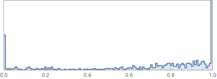
It is also called as electronic noise because it arises in amplifiers or detectors. Gaussian noise caused by natural sources such as thermal vibration of atoms and discrete nature of radiation of warm objects . Gaussian noise generally disturbs the gray values in digital images. That is why Gaussian noise model essentially designed and characteristics by its PDF or normalizes histogram with respect to gray value.
Salt and Pepper Noise:
Salt and Pepper Noise:
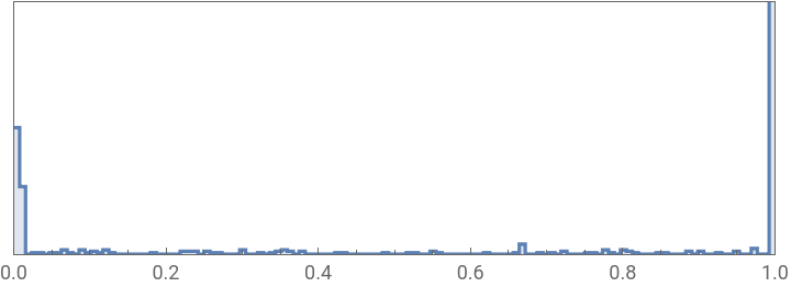
This is also called data drop noise because statistically its drop the original data values. However the image is not fully corrupted by salt and pepper noise instead of some pixel values are changed in the image. Although in noisy image, there is a possibilities of some neighbours does not changed.
Photon Noise (Poisson Noise):
Photon Noise (Poisson Noise):
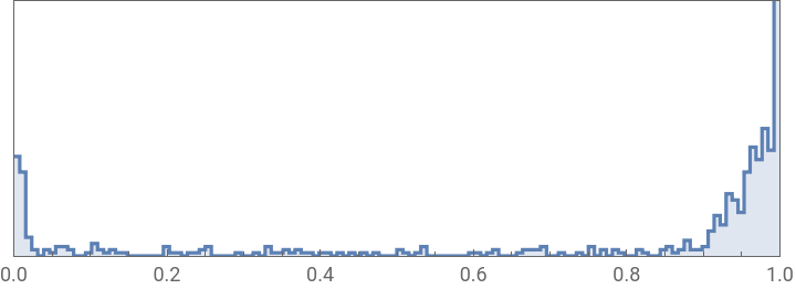
The appearance of this noise is seen due to the statistical nature of electromagnetic waves such as x-rays, visible lights and gamma rays. The x-ray and gamma ray sources emitted number of photons per unit time. These rays are injected in patient’s body from its source, in medical x rays and gamma rays imaging systems. These sources are having random fluctuation of photons. Result gathered image has spatial and temporal randomness. This noise is also called as quantum (photon) noise or shot noise.
Noise Add Codes
Noise Add Codes
In[]:=
addGaussian[img_,thresh_]:=ImageEffect[img,{"GaussianNoise",thresh}]addPoisson[img_,thresh_]:=ImageEffect[img,{"PoissonNoise",thresh}]addSaltPepper[img_,thresh_]:=ImageEffect[img,{"SaltPepperNoise",thresh}]
In[]:=
cleanOutput=Keys@trainingSubset[[1;;10]]
Out[]=
,

,

,

,

,

,

,

,

,


In[]:=
noisyInputG=addGaussian[#,0.2]&/@cleanOutputnoisyInputP=addPoisson[#,0.2]&/@cleanOutputnoisyInputSP=addSaltPepper[#,0.2]&/@cleanOutput
Out[]=
,

,

,

,

,

,

,

,

,


Out[]=
,

,

,

,

,

,

,

,

,


Out[]=
,

,

,

,

,

,

,

,

,


Image histogram visualization
Image histogram visualization
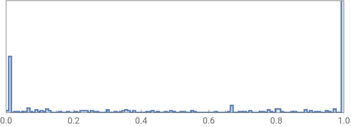
Clean image
Clean image
In[]:=
ImageHistogram[cleanOutput[[1]]]
Out[]=
Salt and Pepper noise image
Salt and Pepper noise image
In[]:=
ImageHistogram[noisyInputSP[[1]]]
Out[]=
Gaussian noise image
Gaussian noise image
In[]:=
ImageHistogram[noisyInputG[[1]]]
Out[]=
Poisson noise Image
Poisson noise Image
In[]:=
ImageHistogram[noisyInputP[[1]]]
Out[]=
Different Noise adding to the dataset
Different Noise adding to the dataset
In[]:=
trainingImagesG=AssociationMap[addGaussian[#,.2]&,Keys[trainingSubset]];testImagesG=AssociationMap[addGaussian[#,.2]&,Keys[testSubset]];
In[]:=
trainingImagesP=AssociationMap[addPoisson[#,.2]&,Keys[trainingSubset]];testImagesP=AssociationMap[addPoisson[#,.8]&,Keys[testSubset]];
In[]:=
trainingImagesSP=AssociationMap[addSaltPepper[#,.2]&,Keys[trainingSubset]];testImagesSP=AssociationMap[addSaltPepper[#,.2]&,Keys[testSubset]];
Data Preparation
Data Preparation
In[]:=
trainAssocG=<|"Input"Values[trainingImagesG],"Output"Keys[trainingImagesG]|>;testAssocG=<|"Input"Values[testImagesG],"Output"Keys[testImagesG]|>;
In[]:=
trainAssocP=<|"Input"Values[trainingImagesP],"Output"Keys[trainingImagesP]|>;testAssocP=<|"Input"Values[testImagesP],"Output"Keys[testImagesP]|>;
In[]:=
trainAssocSP=<|"Input"Values[trainingImagesSP],"Output"Keys[trainingImagesSP]|>;testAssocSP=<|"Input"Values[testImagesSP],"Output"Keys[testImagesSP]|>;
Autoencoder U-NET
Autoencoder U-NET
Autoencoders are a specific type of feedforward neural networks where the input is the same as the output. They compress the input into a lower-dimensional code and then reconstruct the output from this representation. The code is a compact “summary” or “compression” of the input, also called the latent-space representation
Layer Definitions
Layer Definitions
Convolutional Block
Convolutional Block
Convolutional Layer
Convolutional Layer
A convolutional layer contains a set of filters whose parameters need to be learned. The height and weight of the filters are smaller than those of the input volume. Each filter is convolved with the input volume to compute an activation map made of neurons. The output volume of the convolutional layer is obtained by stacking the activation maps of all filters along the depth dimension.
Pooling Layer
Pooling Layer
A pooling layer is usually incorporated between two successive convolutional layers. The pooling layer reduces the number of parameters and computation by down-sampling the representation. The pooling function can be max or average. Max pooling is commonly used as it works better .
Batchnormalization
Batchnormalization
To increase the stability of a neural network, batch normalization normalizes the output of a previous activation layer by subtracting the batch mean and dividing by the batch standard deviation.
In[]:=
conv[n_]:=NetChain[{ConvolutionLayer[n,3,"PaddingSize"{1,1}],Ramp,BatchNormalizationLayer[]}];pool:=PoolingLayer[{2,2},2];
Deconvolutional Block
Deconvolutional Block
U-NET Network
U-NET Network
Network Training
Network Training
Results
Results
Evaluation
Evaluation
Gaussian Denoise
Gaussian Denoise
Noised distance:
Denoised distance:
The noised image had an Image Distance with the original image (taking 2 standard errors) between [5.595,5.603] while the denoised image had an Image distance of [5.58,5.66]. As one range overlaps the other we cannot conclude the denoised images improved the noisy images.
Salt And Peper
Salt And Peper
Noised distance:
The noised image had an Image Distance with the original image (taking 2 standard errors) between [8.67,8.68] while the denoised image had an Image distance of [5.58,5.65]. This new range is way apart from the noisy range of image distance, so we conclude the denoiser improved the image.
Poisson Noise
Poisson Noise
Noised distance:
Denoised distance:
The noised image had an Image Distance with the original image (taking 2 standard errors) between [5.16,5.28] while the denoised image had an Image distance of [5.95,6.03]. And this denoiser seems to make the image worst than before.
Conclusion
Conclusion
Further Work
Further Work
It is possible to improve the Autoencoder performance on the other types of noise y we make a deeper neural net, try bigger datasets or train over more epoch.
Keywords
Keywords
◼
U-NET
◼
Autoencoders
◼
Denoising
◼
MNIST
Acknowledgment
Acknowledgment
Mentor: Wenzhen Zhu
References
References
◼
Image denoising review: From classical to state-of-the-art approaches. Bhawna Goyala, Ayush Dograb, Sunil Agrawala, B.S. Sohic Apoorav Sharmaa.
◼
A REVIEW PAPER: NOISE MODELS IN DIGITAL IMAGE PROCESSING, Ajay Kumar Boyat and Brijendra Kumar Joshi, Signal & Image Processing : An International Journal (SIPIJ) Vol.6, No.2, April 2015
◼
Aparna Vyas, Soohwan Yu, Joonki Paik (2017 )Multiscale Transforms with Application to Image Processing. Signals and Communication Technology. Springer