Andrew Moylan, formerly of Wolfram’s Technical Communication and Strategy group, wrote a blog in 2011 on stabilizing an inverted pendulum in two dimensions (https://blog.wolfram.com/2011/01/19/stabilized-inverted-pendulum/) and a follow-on blog on stabilizing multiple stacked pendula, again in two dimensions (https://blog.wolfram.com/2011/03/01/stabilized-n-link-pendulum/). He promised another follow-on blog about stabilizing the inverted spherical pendulum in three dimensions, but that blog never appeared to the best of my knowledge.
Stabilizing the inverted spherical pendulum in three dimensions is of interest for stabilizing upright robots, rockets, and in other systems.
I attempted his method on the spherical pendulum and encountered difficulties. I am posting this notebook as an invitation to discuss and resolve these difficulties.
The first difficulty is that the output of StateSpaceModel does not appear to have the correct form, and the second difficulty is that the gains computation seems not to halt.
Moylan’s method has the following steps, all straightforwarda:
1
.(easy) Write full non-linear equations of motion in Euler-Lagrange form
2
.(issue) Linearize the equations about the unstable equilibrium of the inverted state via Wolfram’s StateSpaceModel
3
.(issue) Compute the gain matrix of a Linear Quadratic Regulator via Wolfram’s LQRegulatorGains.
4
.(done) Animate a trajectory of an instance of the problem
In the following, I pursue Moylan’s presentation closely, just in 3 dimensions instead of in 2.
Non-Linear Equations of Motion
Non-Linear Equations of Motion
Global Constants
Global Constants
Elementary three-vectors
In[1]:=
ClearAll[o,e1,e2,e3];o={0,0,0};e1={1,0,0};e2={0,1,0};e3={0,0,1};
Acceleration of Earth’s gravitation; length of the pendulum as a thin rod; mass of the rod.
In[3]:=
ClearAll[d,m,g];g=9.81;m=1;d=1;
Coordinate System
Coordinate System
Think of the rod as anchored at its base in an idealized, frictionless, non-locking spherical joint free to slide on a level, flat plane. The generalized coordinates of the point of contact are and . Two angles of the standard spherical coordinate system describe the tilt of the rod: co-latitude θ — angle from vertical, and azimuth ϕ on the plane.
x
y
There are four degrees of freedom. The first-order state-space representation thus has eight variables: four generalized coordinates , , θ, ϕ, and four generalized velocities , yd, θd, ϕd, with the “d” denoting the usual “overdot.”
x
y
xd
Potential energy
Potential energy
Proportional to the height of the center of mass (CM) of the rod above the plane.
In[5]:=
ClearAll[V];V[{x_,y_,θ_,ϕ_,xd_,yd_,θd_,ϕd_}]:=mgCos[θ];
d
2
Kinetic Energy
Kinetic Energy
There are two addends: kinetic energy of translation of the CM in the inertial , , frame and kinetic energy of rotation about the CM.
X
Y
Z
In[7]:=
ClearAll[MI];MI=m;(*momentofinertiaofathinrod*)
1
12
2
d
Angular velocity measured in the inertial frame:
In[9]:=
ClearAll[ω];ω[{x_,y_,θ_,ϕ_,xd_,yd_,θd_,ϕd_}]:=+;
2
θd
2
ϕd
2
Sin[θ]
The CM of the rod in the inertial frame is at position
x[t]+ d 2 |
y[t]+ d 2 |
d 2 |
The following computation ensures the inertial velocities of the CM:
In[11]:=
With{drules={x[t]->x,y[t]->y,θ[t]->θ,ϕ[t]->ϕ,x'[t]->xd,y'[t]->yd,θ'[t]->θd,ϕ'[t]->ϕd}},Withvax=EchoDx[t]+Sin[θ[t]]Cos[ϕ[t]],t/.drules,vay=EchoDy[t]+Sin[θ[t]]Sin[ϕ[t]],t/.drules,vaz=EchoDCos[θ[t]],t/.drules,Null
d
2
d
2
d
2
»
xd+θdCos[θ]Cos[ϕ]-ϕdSin[θ]Sin[ϕ]
1
2
1
2
»
yd+ϕdCos[ϕ]Sin[θ]+θdCos[θ]Sin[ϕ]
1
2
1
2
»
-θdSin[θ]
1
2
Manually copy inertial velocities into the expression for kinetic energy (this seems the most convenient way to get them into a function-like expression):
In[12]:=
ClearAll[T];T[{x_,y_,θ_,ϕ_,xd_,yd_,θd_,ϕd_}]:=m+++MI(+);
1
2
2
xd+θdCos[θ]Cos[ϕ]-ϕdSin[θ]Sin[ϕ]
1
2
1
2
2
yd+ϕdCos[ϕ]Sin[θ]+θdCos[θ]Sin[ϕ]
1
2
1
2
2
-θdSin[θ]
1
2
1
2
2
θd
2
ϕd
2
Sin[θ]
Generalized Forces
Generalized Forces
The generalized forces that can do work applied to virtual displacements δ and δ are just the actual forces [t],[t].
x
y
f
x
f
y
Generalized Torques
Generalized Torques
The torques of [t],[t] are applied at the point of contact, the spherical joint. Thus they do no virtual work applied to virtual displacements δθ and δϕ (I am not fully convinced of this point, but numerical simulation and reading of the literature supports it).
f
x
f
y
Euler-Lagrange Equations
Euler-Lagrange Equations
The Euler-Lagrange equations follow via Wolfram symbolics:
In[14]:=
ClearAll[L,x,y,θ,ϕ,fx,fy,Leqns];L[{x_,y_,θ_,ϕ_,xd_,yd_,θd_,ϕd_}]:=T[{x,y,θ,ϕ,xd,yd,θd,ϕd}]-V[{x,y,θ,ϕ,xd,yd,θd,ϕd}];With[{Lcrds={x[t],y[t],θ[t],ϕ[t]}},With[{Lvels=D[Lcrds,t]},With[{Lncnf={fx[t],fy[t],0,0}},Leqns=Flatten@MapThread[{q,v,f}D[D[L[Lcrds~Join~Lvels],v],t]-D[L[Lcrds~Join~Lvels],q]==f,{Lcrds,Lvels,Lncnf}]]]];
Numerical Verification of Free Motion
Numerical Verification of Free Motion
Drop the pendulum from not-quite-upright and just off the X-axis:
In[17]:=
ClearAll[noforce];noforce={0,0};ClearAll[ndsoln];ndsoln=NDSolve[Join[Leqns/.{fx[t]0,fy[t]->0},{x[0]x'[0]θ'[0]0,θ[0]
0.1
},{y[0]==y'[0]==0,ϕ'[0]==0,ϕ[0]==0.1
}],{x,y,θ,ϕ},{t,0,30}]Out[20]=
xInterpolatingFunction,yInterpolatingFunction,θInterpolatingFunction,ϕInterpolatingFunction


In[51]:=
Plot[{ndsoln[[1,1,2]][t],ndsoln[[1,2,2]][t],ndsoln[[1,3,2]][t]/(2π)},{t,1,10},PlotLegends->{"x","y","θ"}]
Out[51]=
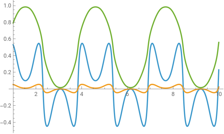


The following animation produces very plausible back and forth swinging motion. The same simulation and animation routines will work when we apply forces.
In[26]:=
ClearAll[DrawSinglePendulum3D,AnimatePendulum3D,SimulatePendulum3D,t];DrawSinglePendulum3D[{x_,y_,θ_,ϕ_}]:=With[{vu=3,axisLabelStyle=textStyle[text,Red,Bold,18,FontFamily"Courier New"]},With[{floor=Polygon[{{-vu,-vu,0},{vu,-vu,0},{vu,vu,0},{-vu,vu,0}}]},Show[Graphics3D[{{Yellow,Opacity[.075],floor},{Blue,Opacity[.1],Cylinder[{{x,y,0},{x,y,0.01}},.5]},{Orange,Cylinder[{{x,y,0},{x+dSin[θ]Cos[ϕ],y+dSin[θ]Sin[ϕ],dCos[θ]}},0.05]}}],AxesTrue,AxesLabelaxisLabelStyle/@{"X","Y","Z"},PlotRange{{-vu,vu},{-vu,vu},{-vu,vu}}]]];AnimatePendulum3D[rules_]:=Animate[With[{cartx=(x/.rules)[u],carty=(y/.rules)[u],φ1=(θ/.rules)[u],φ2=(ϕ/.rules)[u]},DrawSinglePendulum3D[{cartx,carty,φ1,φ2}]],{u,0,Max[First[x/.rules]]},DefaultDuration15,AnimationRunningFalse,SaveDefinitions->True];SimulatePendulum3D[{fxi_,fyi_}]:=With[{ndsoln=NDSolve[Join[Leqns/.{fx[t]fxi,fy[t]->fyi},{x[0]x'[0]0,θ[0]
0.3
,
θ'[0]0},{y[0]==y'[0]==0,ϕ[0]==0.3
,ϕ'[0]==0}],{x,y,θ,ϕ},{t,0,30}]},Module[{vu=3},Column[{Plot[{x[t]/.First@ndsoln,y[t]/.First@ndsoln},{t,0,30},PlotLegends->{"x(t)","y(t)"}(*,PlotRange->{{-vu,vu},{-vu,vu}}*)],AnimatePendulum3D[First[ndsoln]]}]]];SimulatePendulum3D[noforce]State-Space Model
State-Space Model
Moylan’s 2D pendulum produces a state-space model that looks like this:
Our state-space model exhibits two 8x8 matrices, whereas Moylan’s exhibits one 4x4 matrix. I do not understand this 8x8x2 output and would be grateful for advice. However, no error messages are produced, so it appears to be mechanistically OK. In particular, the linearization of the equations of motion appears sound at a glance.
Gains
Gains
The following computation does not terminate in a reasonable time (hours). Again, I would be grateful for advice.
Control Force
Control Force
We cannot complete this exercise because we cannot harvest the gain matrix!