It was a great pleasure to present this demo at APS 2026 alongside 2025 Nobel Laureate in Physics John Martinis, CTO of Qolab, and my good friend Paul Buttles from Qolab.
A pure qubit state lives on the Bloch sphere – a unit sphere whose poles are and and whose equator holds the superposition states. This document builds the complete computational machinery for rotating the Bloch vector from the north pole to any target point, then measuring that state through the dispersive readout chain that a real cQED experiment uses. Every formula is immediately verified with TransmonLab code: if we cannot compute it, we cannot claim to understand it.
|0〉
|1〉
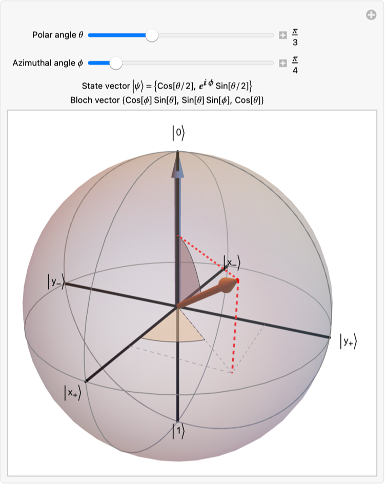
A pure qubit state maps to the Bloch vector =(sinθcosφ,sinθsinφ,cosθ). The ground state sits at the north pole ; the excited state at the south pole . Our task is to rotate from north pole to any target .
|ψ〉=cos(θ/2)|0〉+sin(θ/2)|1〉
φ
R
|0〉
(0,0,1)
|1〉
(0,0,-1)
(θ,φ)
Out[]=
We start with the transmon Hamiltonian and its charge-basis spectrum, then move to Bloch sphere geometry, calibrate pulse amplitudes via Power Rabi, demonstrate arbitrary state preparation, examine decoherence and DRAG corrections, and finally close the loop from qubit to digitizer by generating synthetic IQ measurement data – both final integrated shots for state tomography and time-resolved , traces that reveal the cavity ring-up in real time.
I(t)
Q(t)
The schematic below shows the basic transmon circuit: a Josephson junction shunted by a capacitor, capacitively coupled to a readout resonator.
In[]:=
TransmonCircuitPlot[Background->White]
Out[]=
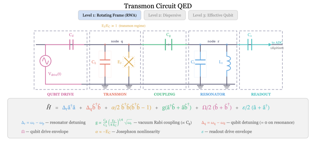
Consider the Hamiltonian as =4--cos with the Cooper-pair number with integer eigenvalues, and ϕ the superconducting phase across the junction. They are canonically conjugate: and =-. Additionally, is the charging energy, is the Josephson energy, and is the gate offset charge. The Hamiltonian can be considered as a quantum rotor (phase) in a cosine potential, minimally coupled to a static “vector potential” that shifts the momentum .
H
2
E
C
n
n
g
E
J
ϕ
n
,=
ϕ
n
n
∂
∂ϕ
E
C
E
J
n
g
n
g
n
The charge basis is denoted as with |n〉=n|n〉. The phase operator acts as a ladder in this basis: |n〉=|n∓1〉. Thus, this implies . Put all of these together, the Hamiltonian can be described in a truncated space, by setting .
{|n〉}
nϵ
n
±
ϕ
cos=(|n〉〈n+1|+|n+1〉〈n|)
ϕ
1
2
∑
n
-<=n<=
n
max
n
max
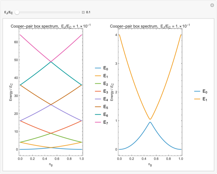
The interactive plot below shows the Cooper-pair box energy spectrum as a function of the ratio EJ/EC. In the transmon regime (EJ/EC >> 1), the energy levels flatten and become insensitive to offset charge, which is the key engineering advantage of the transmon design. The left panel shows 6 levels; the right panel shows only the computational subspace (2 levels).
Out[]=
1. The Target: Points on the Bloch Sphere
1. The Target: Points on the Bloch Sphere
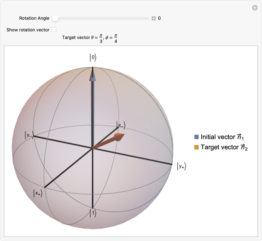
Assume the initial qubit state is represented by the Bloch vector . We now seek a rotation that maps ->. Geometrically, this is a rigid rotation in the plane spanned by and , through the angle between the two vectors. The plane spanned by and is also fully specified by the the vector cross product and . In short, the rotation is given by ×(ArcCos[.]) with unit vectors =.
r
1
r
1
r
2
r
1
r
2
r
1
r
2
r
1
r
2
ℛ
n
1
n
2
n
1
n
2
n
j
r
j
r
j
For two Bloch vectors, visualize the plane spanned by them and also the perpendicular vector defining it:
Out[]=
To reach an arbitrary target from , we need exactly two operations:
(θ,φ)
|0〉
1. FrameRotation["Qubit", ] – sets the rotation axis. This is a virtual Z-gate: zero duration, zero error. The relationship between the Bloch sphere azimuthal angle φ and the frame rotation is =φ+π/2. This follows from the Rodrigues rotation formula: a drive at phase creates axis =(cos,sin,0), and the first point the north pole reaches is ×=(sin,-cos,0). Setting this equal to gives =φ+π/2.
φ
rot
φ
rot
φ
rot
n
φ
rot
φ
rot
n
z
φ
rot
φ
rot
(cosφ,sinφ,0)
φ
rot
2. Drive[Amplitude[a] @ pulse, "Qubit"] – applies the rotation. The amplitude controls the polar angle via the calibration constant .
a
θ
θ=a×
θ
1
The mapping is the key calibration step.
(θ,φ)→(a,)
φ
rot
3. Hardware Parameters and Pulse Design
3. Hardware Parameters and Pulse Design
We define a TransmonSystem with parameters representative of a modern transmon qubit:
In[]:=
sys=TransmonSystem"QubitFrequency"5.10*,"ResonatorFrequency"6.00*,"Anharmonicity"-220*,"Coupling"100*,"CavityLinewidth"1*,"T1"50*,"T2"30*,"OmegaMax"2π*42*,"EpsilonMax"2π*5*,"NMax"5
9
10
9
10
6
10
6
10
6
10
-6
10
-6
10
6
10
6
10
Out[]=
TransmonSystem

Inspect the full set of derived parameters, including the dispersive shift, decay rates:
In[]:=
AssociationThread"","","",Map[sys[#]&,{"Chi","Gamma1","GammaPhi"}]
χ
2π
Γ
1
Γ
ϕ
These are typical values for a transmon in the dispersive regime (Rasmussen et al., arXiv:2103.01225, Table I).
Create a Gaussian pulse for qubit rotations and a FlatTop pulse for readout:
One can define any arbitrary pulse. This pulse is usually called a sech pulse (or sech/tanh pulse), and the technique it’s used for is called Adiabatic Rapid Passage (ARP).
Visualize pulses:
Amplitude Calibration (Theory)
Amplitude Calibration (Theory)
Calculate the rotation angle per unit amplitude:
4. Calibration: Power Rabi Sweep
4. Calibration: Power Rabi Sweep
Define the sweep and run:
Pulse sequence as: run the qubit with Gaussian pulse, then sync and then readout pulse on resonator:
Given transmon system and other features, solve dynamical equations:
Visualize the built-in simulation result, showing the population dynamics:
Summary so far:
Run the simulation with the QubitOnly model to obtain the Bloch trajectory:
Compare simulated and analytic Bloch vectors:
Comparing final Bloch vectors:
The error is small, limited by the truncated Gaussian envelope. The two arrows are nearly indistinguishable – the two-operation recipe works for arbitrary targets.
Measurement in different basis
Measurement in different basis
Solve dynamical equation:
Visualize the evolution of the Bloch sphere:
Find density matrix for the case of Pauli-Z measurement:
Find density matrix for the case of Pauli-X measurement:
Calculate probabilities for computational basis:
Calculate probabilities for x-basis :
6. Where is Measurement? From Qubit to Digitizer (IQ Data)
6. Where is Measurement? From Qubit to Digitizer (IQ Data)
Everything we have done so far operates at the level of the Bloch vector – deterministic, clean, and noiseless. But a real experiment ends at the digitizer: the qubit state is encoded in the amplitude and phase of a microwave signal leaking from the cavity, which is amplified, mixed down, and digitized into I and Q quadratures. Each single shot yields one (I, Q) point, and the qubit state must be inferred from statistics over many shots.
Setting Up the Readout
Setting Up the Readout
Here’s the key physics. The cavity equation of motion depends on the qubit state:
Create a DispersiveReadout object from our system and readout pulse:
Visualize the cavity pointer states – the IQ-plane trajectories that the cavity field follows depending on the qubit state:
The two spirals in the IQ plane separate over time as the dispersive shift χ rotates them in opposite directions. The distance between the pointer states at the end of the readout determines the signal-to-noise ratio.
The pointer states tell us where the signal will land on average – but a real experiment never sees these clean spirals. Each single shot of the measurement produces one (I, Q) point drawn from a noisy cloud around the pointer state, because quantum measurement is intrinsically stochastic and the amplification chain adds its own noise on top. The qubit may also decay during readout, blurring the boundary between the two clouds further. To learn anything about the prepared state, we must repeat the experiment many times and build up statistics: a histogram of single-shot (I, Q) outcomes whose cluster positions, shapes, and relative weights encode the qubit populations and coherences.
TransmonLab’s IQTrajectory object models exactly this: it runs a stochastic simulation of the qubit–cavity system for each shot, drawing quantum jumps and measurement noise from their proper distributions, and returns the resulting (I, Q) record. We can then feed these synthetic single-shot data into IQAnalysis, which performs Gaussian mixture fitting, computes assignment fidelities, and reconstructs the Bloch vector via tomography – the same pipeline one would run on data from a real dilution refrigerator.
State Tomography
State Tomography
Since the target state is not an eigenstate of any Pauli operator, the pre-rotations for tomography are nontrivial. Compute them by applying the basis-change rotations to the state vector:
Generate three-basis IQ measurements with these pre-rotated initial states:
Plot the time-resolved I(t) and Q(t) records for the first two shots in each measurement basis. These raw traces show the cavity ring-up signal as it evolves during the readout window:
Plot the running integral of the I and Q records. As the integration window grows, the signal accumulates and the two qubit-state clusters separate:
Visualize the integrated IQ trajectories in 3D (time × I × Q) for each measurement basis. Each thin line is one shot evolving over time:
Project the trajectories onto the IQ plane. The blue dots mark the final integrated (I, Q) value for each shot – these are the single-shot measurement outcomes that feed into the analysis:
Plot the density of final IQ measurement points for each basis as smooth histograms. The two-blob structure reflects the qubit being projected into either the ground or excited state on each shot:
Feed the measurement data into IQAnalysis, which performs Gaussian mixture fitting, computes assignment fidelities, and reconstructs the Bloch vector:
Compare the reconstructed Bloch vector to the target:
The reconstructed state sits close to the target. The small discrepancy is the combined effect of finite shot noise, decoherence during readout, and the stochastic nature of quantum measurement – exactly what happens in a real experiment.
Visualize the reconstructed Bloch vector on the Bloch sphere alongside the target, showing the tomographic result:
IQAnalysis classifies single shots by projecting each (I, Q) point onto the optimal discriminant axis connecting the two Gaussian centroids, then applying a threshold. The Mahalanobis distance quantifies how well-separated the two clouds are after accounting for their shape and spread: it stretches and rotates the IQ plane so that both Gaussian blobs become unit circles, then measures ordinary Euclidean distance. A larger Mahalanobis distance means better readout fidelity. The Bloch distribution plots below show the statistical uncertainty in the reconstructed Bloch vector components.
Plot the marginal distributions of the reconstructed Bloch vector components (Rx, Ry, Rz), showing the uncertainty from finite shot noise:
Plot the radial distribution of the Bloch vector length, which quantifies how close the reconstructed state is to a pure state:
7. Real Experimental Data
7. Real Experimental Data
We now repeat the same analysis on real hardware data from the Qolab cloud quantum computing platform, using the same target state to compare simulation and experiment.
Credentials from Qolab (contact Qolab if you are interested to get token):
Send a query to Qolab and get IQ result:
Visualize IQ results:
Analyze IQ results (with no info from hardware, for now):
View the full diagnostics: assignment fidelity, Gaussian fit parameters, SNR, and classification thresholds:
Find the estimated Bloch vector:
Plot it:
Plot the marginal distributions of the reconstructed Bloch vector components (Rx, Ry, Rz), showing the uncertainty from finite shot noise:
Plot the radial distribution of the Bloch vector length, which quantifies how close the reconstructed state is to a pure state:
8. Effect of Decoherence
8. Effect of Decoherence
Define the ideal system (effectively infinite coherence):
Simulate ideal case and the case with decohernece:
State Fidelity After Preparation
State Fidelity After Preparation
9. DRAG Pulses for Leakage Suppression
9. DRAG Pulses for Leakage Suppression
Build drive-only sequences for both Gaussian and DRAG at the π-pulse amplitude. No readout is included – the Duffing model’s qubit-cavity coupling would introduce readout backaction that obscures the leakage comparison:
Compare Gaussian and DRAG pulse shapes:
Run both sequences through the 3-level Duffing model to compare leakage:
Compare populations and leakage against the ideal π pulse:
Where This Leaves Us
Where This Leaves Us
We have built a complete computational pipeline for single-qubit state preparation and measurement:
Initialization
Initialization
CITE THIS NOTEBOOK
CITE THIS NOTEBOOK
Transmon cQED: Wolfram x Qolab collaboration
by Mohammad Bahrami
Wolfram Community, STAFF PICKS, March 19, 2026
https://community.wolfram.com/groups/-/m/t/3666356
by Mohammad Bahrami
Wolfram Community, STAFF PICKS, March 19, 2026
https://community.wolfram.com/groups/-/m/t/3666356