ORIGINAL ARTICLE: Hui, C., Pyšek, P. & Richardson, D.M. Disentangling the relationships among abundance, invasiveness and invasibility in trait space. npj biodivers 2, 13 (2023). DOI: https://doi.org/10.1038/s44185-023-00019-1
Article Abstract: Identifying conditions and traits that allow an introduced species to grow and spread, from being initially rare to becoming abundant (defined as invasiveness), is the crux of invasion ecology. Invasiveness and abundance are related but not the same, and we need to differentiate these concepts. Predicting both species abundance and invasiveness and their relationship in an invaded community is highly contextual, being contingent on the community trait profile and its invasibility. We operationalised a three-pronged invasion framework that considers traits, environmental context, and propagule pressure. Specifically, we measure the invasiveness of an alien species by combining three components (performance reflecting environmental suitability, product of species richness and the covariance between interaction strength and species abundance, and community-level interaction pressure); the expected population growth rate of alien species simply reflects the total effect of propagule pressure and the product of their population size and invasiveness. The invasibility of a community reflects the size of opportunity niches (the integral of positive invasiveness in the trait space) under the given abiotic conditions of the environment. Both species abundance and the surface of invasiveness over the trait space can be dynamic and variable. Whether an introduced species with functional traits similar to those of an abundant species in the community exhibits high or low invasiveness depends largely on the kernel functions of performance and interaction strength with respect to traits and environmental conditions. Knowledge of the covariance between interaction strength and species abundance and these kernel functions, thus, holds the key to accurate prediction of invasion dynamics.
The code is prepared by C. Hui using Mathematica 12.0 (02/11/2022; Wolfram, Inc.). The code running requires about 5 min to complete on a Dell OptiPlex 7060 with Intel(R) Core(TM) i7-8700 CPU and 16 GB RAM. Below, we provide a brief introduction to the code structure.
The model implements an open ecological community under persistent once-off biological invasions. All residing species within the community, also including the introduced alien species, engage in resource competition with an interaction strength determined by the traits of the two involved species. The intrinsic rate of growth of each species is also trait dependent. In a nutshell, a species' trait position in the community trait profile determines its performance and interactions with other species. For jargons and expanded code, please see Table 1 and main text, as well as Hui et al. 2021 ( https://doi.org/10.1007/s10530-021-02484-w ).
First, we define the kernel functions of r (intrinsic rate of growth) and a (interaction strength [competition] between two species) in the two dimensional trait space (x, y). Coefficients siga and sigr are related to the specific shapes of the kernel functions. Inner functions of Mathematica are intutitve; chop[] removes small positive numbers close to zeros, Exp[] is the exponential function, If[] is for conditional, and Sqrt[] is for square root calculation; see Mathematica Help for more details.These two parameterised kernel functions are for the left plot in Fig.2.
In[]:=
siga=0.03;sigr=0.35;a[x1_,y1_,x2_,y2_]:=Chop[Exp[-((x1-x2)^2+(y1-y2)^2)/(2siga)]];r[x1_,y1_]:=If[Sqrt[((x1)^2+(y1)^2)]<1,0.5,0];
Second, the introduction events of alien species are pre-defined using a Poisson process (with u the intensity [number of introduction events per unit of time]) to specify the timing of each event, with the trait of the introduced species (x, y) randomly drawn in the trait space (-1<x<1, -1<y<1). A total of 10,000 introduction events are prepared and will be sequentially introduced into the community at the time according to vector tt. Please see Mathematica Help for inner functions (PoissonProcess[], RandomFunction[], Dimensions[], and RandomReal[]).
In[]:=
u=1.2;tt=RandomFunction[PoissonProcess[u],{0,10000}]["Path"][[All,1]];tn=Dimensions[tt][[1]];x=RandomReal[{-1,1},tn];y=RandomReal[{-1,1},tn];
Third, the following is the main part of the code. It specifies the ordinary differential equations (ODEs) for survived residents and newly introduced: comm describes the generic Lotka-Volterra model with trait-mediated performance and interactions (r and a), where set is the dynamic species identity set, len the number of species in the community, and abu the abundance of each species in the community. The ODEs are then solved by NDSolve[] between two introduction events and the solution assigned to sol. All of these are written within a loop (Do[] for k introduction events; for demonstration, we consider a number of k = tmax introduction events here but can be modified if needed. A species is considered extinct if its standing population density n is less than a threshold (0.01; can be modified). Note, n records population densities for all species, whereas abu only for those currently in the community.
In[]:=
Clear[t]set={1};len[1]=Length[set];spp[0]=set;abu[0]={0.01};comm=Flatten[Table[{n[i]'[t]n[i][t](r[x[[i]],y[[i]]]-Sum[a[x[[i]],y[[i]],x[[j]],y[[j]]]n[j][t],{j,set}]),n[i][tt[[1]]]0.01},{i,set}]];sol=NDSolve[comm,Table[n[i],{i,set}],{t,tt[[1]],tt[[2]]}];spp[1]=set;abu[1]=Evaluate[Table[n[i][tt[[2]]],{i,set}]/.sol][[1]];tmax=1000;Monitor[Do[{ext=Table[If[n[i][tt[[k]]]<0.01,True,False],{i,set}]/.sol[[1]];pos=Flatten[Position[ext,True],1];set=Union[Complement[set,set[[pos]]],{k}];len[k]=Length[set];comm=Flatten[Table[{n[i]'[t]n[i][t](r[x[[i]],y[[i]]]-Sum[a[x[[i]],y[[i]],x[[j]],y[[j]]]n[j][t],{j,set}]),n[i][tt[[k]]]If[ik,0.01,n[i][tt[[k]]]/.sol[[1]]]},{i,set}]];sol=NDSolve[comm,Table[n[i],{i,set}],{t,tt[[k]],tt[[k+1]]},Method{"EquationSimplification""Residual"}];spp[k]=set;abu[k]=Evaluate[Table[n[i][tt[[k+1]]],{i,set}]/.sol][[1]]},{k,2,tmax}],k]
Additional metrics can be computed by the following code, which records each species time of entry, time of extirpation, duration, and abundance dynamics during its residence time in the community:
In[]:=
Do[{time=Flatten[Position[Table[Length[Cases[spp[i],k]],{i,tmax}],1]];tbegin[k]=Min[tt[[time]]];tend[k]=Max[tt[[time]]];life[k]=tend[k]-tbegin[k];ab=Flatten[Table[abu[t][[Flatten[Position[spp[t],k]]]],{t,time[[1]],time[[-1]]}]];abm[k]=Mean[ab];abme[k]=Median[ab];abma[k]=Max[ab];abp[k]=ab;},{k,1,tmax}]
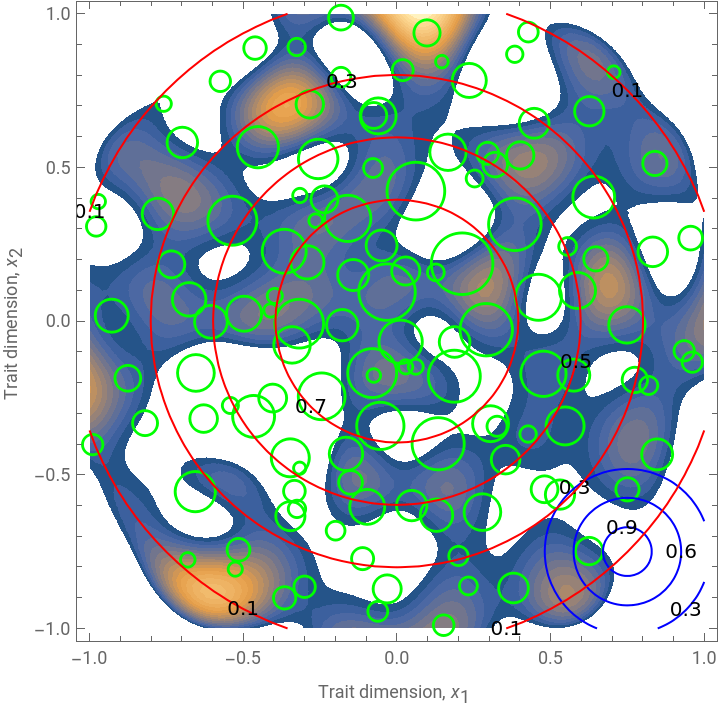
Finally, the following code is for visualisation and will generate the left plot of Fig.2. Specifically, it overlays a number of plots. It visualizes population densities/abundances as green circles, invasiveness as contour surface, kernel function of r as red contour circles, and competition kernel of a as blue contour circles. Please see the legend of Fig.2 for details.
In[]:=
t=tmax;fig1=Graphics[Table[{Green,Thickness[0.0045],Circle[{x[[i]],y[[i]]},0.2Sqrt[abu[t][[Position[spp[t],i][[1]]]][[1]]]]},{i,spp[t]}],FrameTrue,PlotRange{{-1,1},{-1,1}}];fig2=ContourPlot[a[0.75,-0.75,x1,y1],{x1,-1,1},{y1,-1,1},ContourStyleBlue,Contours{0.3,0.6,0.9},PlotRangeAll,ContourLabelsTrue,ContourShadingNone];fig3=Graphics[{Red,Circle[{0,0},1]}];cen=Table[r[xref,yref]-Sum[a[xref,yref,x[[spp[t][[j]]]],y[[spp[t][[j]]]]]abu[t][[j]],{j,len[t]}],{xref,-1,1,0.02},{yref,-1,1,0.02}];tx=ListContourPlot[cen,DataRange{{-1,1},{-1,1}},Contours20,PlotRange{0,All},ContourStyleNone];Show[tx,fig1,fig2,fig3,FrameLabel{"Trait dimension, ","Trait dimension, "},PlotRange{{-1,1},{-1,1}}]
x
1
x
2
Out[]=
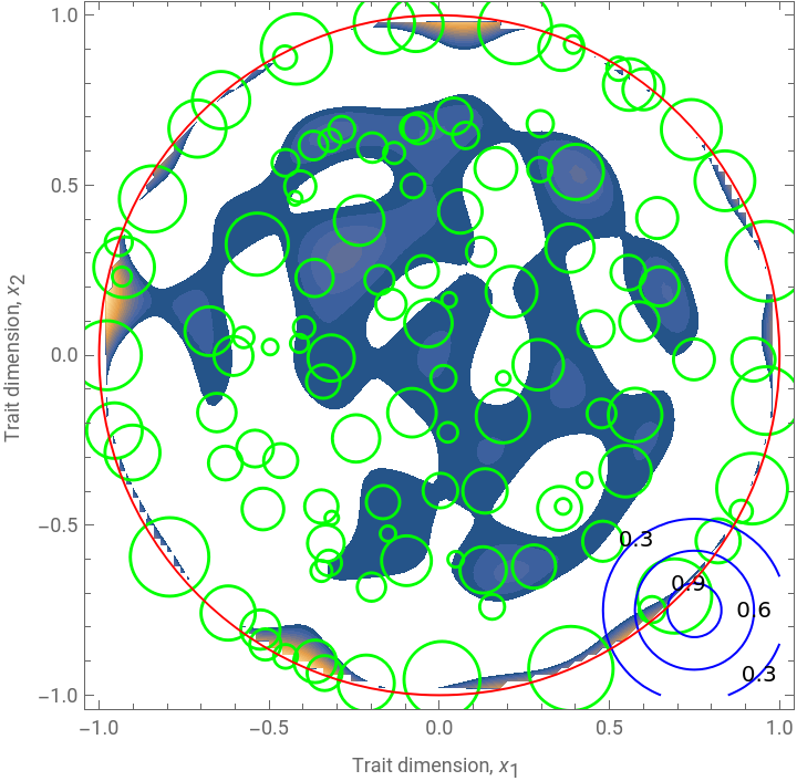
Note, a graphic will be produced from the code above (Fig.2 left).
The following code will produce the right plot in Fig.2. The only difference between the left and the right plot is the kernel function of r. Above, r is a constant within the unit disk; below, r is a Gaussian function centred at the origin of the trait space minus a constant (to sink the intrinsic growth rate surface so that it becomes negative outside the unit disk). The first three steps of the above code are simply lumped together below into one block.
In[]:=
r[x1_,y1_]:=Max[0,Exp[-((x1)^2+(y1)^2)/(2sigr)]-0.1];(*forFig.1Right*)(*Opencommunityassemblyviasequentialspeciesintroductions*)Clear[t]set={1};len[1]=Length[set];spp[0]=set;abu[0]={0.01};comm=Flatten[Table[{n[i]'[t]n[i][t](r[x[[i]],y[[i]]]-Sum[a[x[[i]],y[[i]],x[[j]],y[[j]]]n[j][t],{j,set}]),n[i][tt[[1]]]0.01},{i,set}]];sol=NDSolve[comm,Table[n[i],{i,set}],{t,tt[[1]],tt[[2]]}];spp[1]=set;abu[1]=Evaluate[Table[n[i][tt[[2]]],{i,set}]/.sol][[1]];tmax=1000;Monitor[Do[{ext=Table[If[n[i][tt[[k]]]<0.01,True,False],{i,set}]/.sol[[1]];pos=Flatten[Position[ext,True],1];set=Union[Complement[set,set[[pos]]],{k}];len[k]=Length[set];comm=Flatten[Table[{n[i]'[t]n[i][t](r[x[[i]],y[[i]]]-Sum[a[x[[i]],y[[i]],x[[j]],y[[j]]]n[j][t],{j,set}]),n[i][tt[[k]]]If[ik,0.01,n[i][tt[[k]]]/.sol[[1]]]},{i,set}]];sol=NDSolve[comm,Table[n[i],{i,set}],{t,tt[[k]],tt[[k+1]]},Method{"EquationSimplification""Residual"}];spp[k]=set;abu[k]=Evaluate[Table[n[i][tt[[k+1]]],{i,set}]/.sol][[1]]},{k,2,tmax}],k]
The code below is for visualisation of the right plot of Fig.2; specifics are the same as above and detailed in the figure legend.
In[]:=
t=tmax;fig1=Graphics[Table[{Green,Thickness[0.0045],Circle[{x[[i]],y[[i]]},0.2Sqrt[abu[t][[Position[spp[t],i][[1]]]][[1]]]]},{i,spp[t]}],FrameTrue,PlotRange{{-1,1},{-1,1}}];fig2=ContourPlot[a[0.75,-0.75,x1,y1],{x1,-1,1},{y1,-1,1},ContourStyleBlue,Contours{0.3,0.6,0.9},PlotRangeAll,ContourLabelsTrue,ContourShadingNone];fig3=ContourPlot[r[x1,y1],{x1,-1,1},{y1,-1,1},Contours{0.1,0.3,0.5,0.7,0.9},ContourStyleRed,PlotRangeAll,ContourLabelsTrue,ContourShadingNone];cen=Table[r[xref,yref]-Sum[a[xref,yref,x[[spp[t][[j]]]],y[[spp[t][[j]]]]]abu[t][[j]],{j,len[t]}],{xref,-1,1,0.02},{yref,-1,1,0.02}];tx=ListContourPlot[cen,DataRange{{-1,1},{-1,1}},Contours20,PlotRange{0,All},ContourStyleNone];Show[tx,fig1,fig2,fig3,FrameLabel{"Trait dimension, ","Trait dimension, "},PlotRange{{-1,1},{-1,1}}]
x
1
x
2
Out[]=
CITE THIS NOTEBOOK
CITE THIS NOTEBOOK
Disentangling the relationships among abundance, invasiveness and invasibility in trait space
by Cang Hui
Wolfram Community, STAFF PICKS, June 13, 2023
https://community.wolfram.com/groups/-/m/t/2936678
by Cang Hui
Wolfram Community, STAFF PICKS, June 13, 2023
https://community.wolfram.com/groups/-/m/t/2936678