CITE THIS NOTEBOOK: Graph/cluster states, and measurement-based quantum computation by Mads Bahrami. Wolfram Community MAR 2022.
A very unique approach to quantum computation is the measurement-based quantum computation, which depends on sequence of local measurements on an entangled state, called the graph state. In this short computational essay, I explore the graph state (also called the cluster state), its implementation in the Wolfram Mathematica, and some applications for the teleportation-based quantum computation.
Special thanks to my friend and colleague, Michael Trott (Wolfram Research), who brought this interesting topic to my attention. There are many good references out these on this topic, a few among them that I used in this computational essay are:
◼
Section 12.1 and 12.2 of this book: Quantum Information Processing, Quantum Computing, and Quantum Error Correction
Graph state
Graph state
We consider only the binary graph states, where there is not self-loop, only single or no edge between two vertices, and all edges have the same weight.
In[]:=
g=TreeGraph[1#&/@Range[2,4],VertexLabels"Name"]
Out[]=
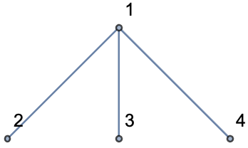
Qubits will be list of vertices:
In[]:=
qubits=VertexList[g]
Out[]=
{1,2,3,4}
Prepare the initial state as by applying Hadamard operators on
⊕n
|+〉
⊕n
|0〉
In[]:=
plus=QuantumOperator[{"H",Length[qubits]}][QuantumState[{"Register",Length[qubits]}]]
Out[]=
QuantumState


For each edge, apply a controlled-Z operator on corresponding vertices. In this way, both graph state and corresponding quantum circuit can be generated
In[]:=
qc=QuantumCircuitOperator[QuantumOperator["CZ",List@@#]&/@EdgeList[g]];qc["Diagram"]
Out[]=
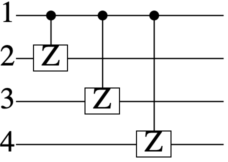
Apply circuit operator on the initial plus state to create the graph state:
In[]:=
qc[plus]
Out[]=
QuantumState

Return the formula of the graph state:
In[]:=
%["Formula"]
Out[]=
1
4
1
4
1
4
1
4
1
4
1
4
1
4
1
4
1
4
1
4
1
4
1
4
1
4
1
4
1
4
1
4
Given a list of vertices adjacent to a vertex, create the corresponding stabilizer generators:
In[]:=
stabilizers=MapIndexed[QuantumOperator["X",#2][QuantumOperator["Z",#1]]&]@AdjacencyList[g]
Out[]=
QuantumOperator,QuantumOperator,QuantumOperator,QuantumOperator


Note that stabilizers[[i]] represents the a stabilizer operator associated with the i-th vertex
Show that the graph state are the stabilizer generators eigenstate
In[]:=
Thread[Equal[Through[stabilizers[qc[plus]]],-qc[plus]]]
Out[]=
{True,True,True,True}
Create the Hamiltonian
In[]:=
-Total[stabilizers]
Out[]=
QuantumOperator

Find the ground state of the Hamiltonian
In[]:=
%["Eigenvectors"][[1]]//QuantumState
Out[]=
QuantumState
Show it is the same as the graph state
In[]:=
%==qc[plus]
Out[]=
True
Generate the graph basis associated with the graph state
In[]:=
graphBasis=Through[(QuantumCircuitOperator[MapIndexed[QuantumOperator["Z",#2]^#1&][#]]["QuantumOperator"]&/@Tuples[{0,1},Length@VertexList[g]])[qc[plus]]];
Show that the graph basis are orthonormal:
In[]:=
DistanceMatrix[graphBasis,DistanceFunctioninnerProduct]==IdentityMatrix[2^Length@VertexList[g]]
Out[]=
True
Show that the graph basis is also complete
In[]:=
Total[outerProduct[#,#]&/@graphBasis]==QuantumOperator["Identity",VertexList[g]]
Out[]=
True
One can automate the generation of graph state, the corresponding quantum circuit, and the stabilizer operators of any graph, as follows
In[]:=
GraphQuantumData[g_Graph]:=Module[{qubits,plus,qc,stabilizers},qubits=VertexList[g];qc=QuantumCircuitOperator[QuantumOperator["CZ",List@@#]&/@EdgeList[g]];plus=QuantumOperator[{"H",Length[qubits]}][QuantumState[{"Register",Length[qubits]}]];stabilizers=QuantumOperator["X",{#1}][QuantumOperator["Z",#2]]&@@@Transpose[Through[{VertexList,AdjacencyList}[g]]];<|"GraphState"->qc[plus],"GraphCircuit"->qc,"StabilizerGenerators"->stabilizers|>];
Note that given a graph, one can use the named quantum state “Graph” in our framework, which returns the graph state:
In[]:=
QuantumState[{"Graph",g}]==GraphQuantumData[g]["GraphState"]
Out[]=
True
Grid graph
Grid graph
Grid graph, as another example
In[]:=
g=GridGraph[{2,4},VertexLabels"Name"]
Out[]=
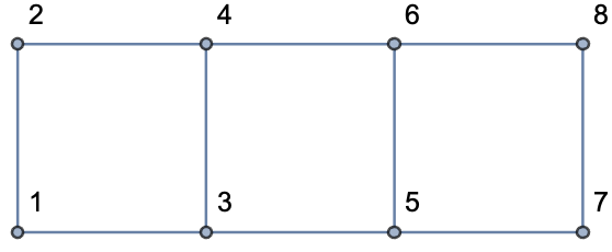
Generate the corresponding quantum data of graph:
In[]:=
gridG=GraphQuantumData[g];
The corresponding circuit of the graph:
In[]:=
gridG["GraphCircuit"]["Diagram"]
Out[]=
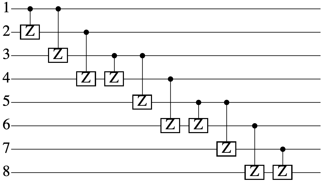
Show the graph state is the eigenstate of stabilizer generators
Corresponding graph basis:
Local complementation
Local complementation
Given a vertex v, in the neighbourhood of v, remove edges if they are present, and adds any edges are missing (this is also called as “local complementation of a vertex”)
Generate a random graph with 5 vertices and 6 edges:
Find the local complementation wrt the vertex 5:
Given a vertex v of a graph g, find a local unitary operator that transforms g into its local complementation of vertex v:
Generate a graph state by applying unitary of local complementation:
Since the unitary operator for the local complementation has sqrt of some other operators etc, we should look into chopped numerical values (to remove eg the machine precision error etc) and compare the quantum state we get from action of unitary on the initial graph state, with the quantum graph state we get directly from the new graph.
Teleportation of the quantum state though a linear chain of qubits
Teleportation of the quantum state though a linear chain of qubits
Consider this scenario: qubit-1 is prepared in a generic state ψ0. We plan to teleport it to qubit-4 by measuring Pauli-X on qubits 1-3
Prepare qubits 2-3 in a graph state
The initial state of qubit-1 (a generic state)
Apply CZ on qubit 1 and 2 (add an edge between vertex 1 and 2), then measure Pauli-X on qubits 1-3
Given post-measurement states, trace out qubits 1-3, and get the state of qubit-4
Note given three measurements, each one two outcomes, we get 8 different realizations for outcomes.
Test for all combination of measurement results, the post-measurement state of qubit-4 is what we expected (we added the factor 8 only for normalization):
Generalization
Generalization
The initial state of qubit-1 (a generic state)
Implementing an arbitrary one-qubit unitary gate
Implementing an arbitrary one-qubit unitary gate
Define a series of measurement for different angles:
Generate the operator to entangle graph vertices (ie qubits) and combine it with series of qubit measurments:
Given a list of zeroes and ones, post-select the corresponding state after doing all measurements etc
Check for all combination of zeroes of ones for four qubits 1-4 (all possible measurement results), the result of applying about unitary is the same as the reduced state of measurement
Equatorial-basis measurements on grid graphs
Equatorial-basis measurements on grid graphs
If measuring only in the XY-plane of Bloch sphere, with ξ the angle from x-axis, eigensysem is:
Create a 2x4 grid graph:
Make it open-ended, by removing the edge of two last vertices:
Generate corresponding operator circuit that entangles neighboring qubits by CZ
Test that above circuit on |++> is the same as identity:
Given above result, find the relative phase between two states (note two states are the same, only a difference in phase)
Get the final state using the graph state (czij plusN[8]) and project it when first 6 qubits are in the plus state:
Test if the final state is the same as |++>:
Given above result, find the relative phase between two states (note two states are the same, only a difference in phase)
Now instead of measuring Pauli-X on qubits 1-6, let’s measure qubits 1 and 2 along a specific angle in the XY-plan:
Corresponding usual quantum circuit:
Another circuit with the same result:
Test if the final state is the same as the state one gets out of the circuit
Given above result, find the relative phase between two states (note two states are the same, only a difference in phase)
Test if the final state is the same as the state one gets out of the circuit
Given above result, find the relative phase between two states (note two states are the same, only a difference in phase)
Now instead of measuring Pauli-X on qubits 1-6, let’s measure qubits 5 and 6 along a specific angle in the XY-plan:
Test if the final state is the same as the state one gets out of the circuit
Similar test, for the state we obtained manually (manualState)
Given above result, find the relative phase between two states (note two states are the same, only a difference in phase)
Paclet installation
Paclet installation
Install the paclet
Define two functions for the quantum inner and outer products of quantum states