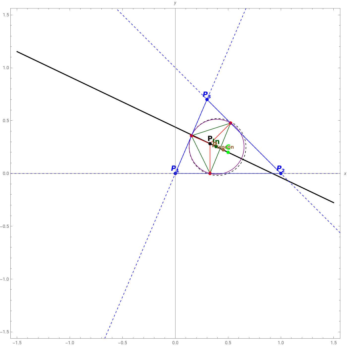
FontenéThirdTheorem::usage="Fontené's third theorem states that if a point and its isogonal conjugate are on a straight line what passes through the circumcenter and incenter of the base triangle, then its pedal circle its tangent to the circle of the 9 points. References: Wolfram MathWorld: Fontené theorems, Pedal circle, Pedal triangle; Personal."
Example 1:
In[]:=
Out[]=


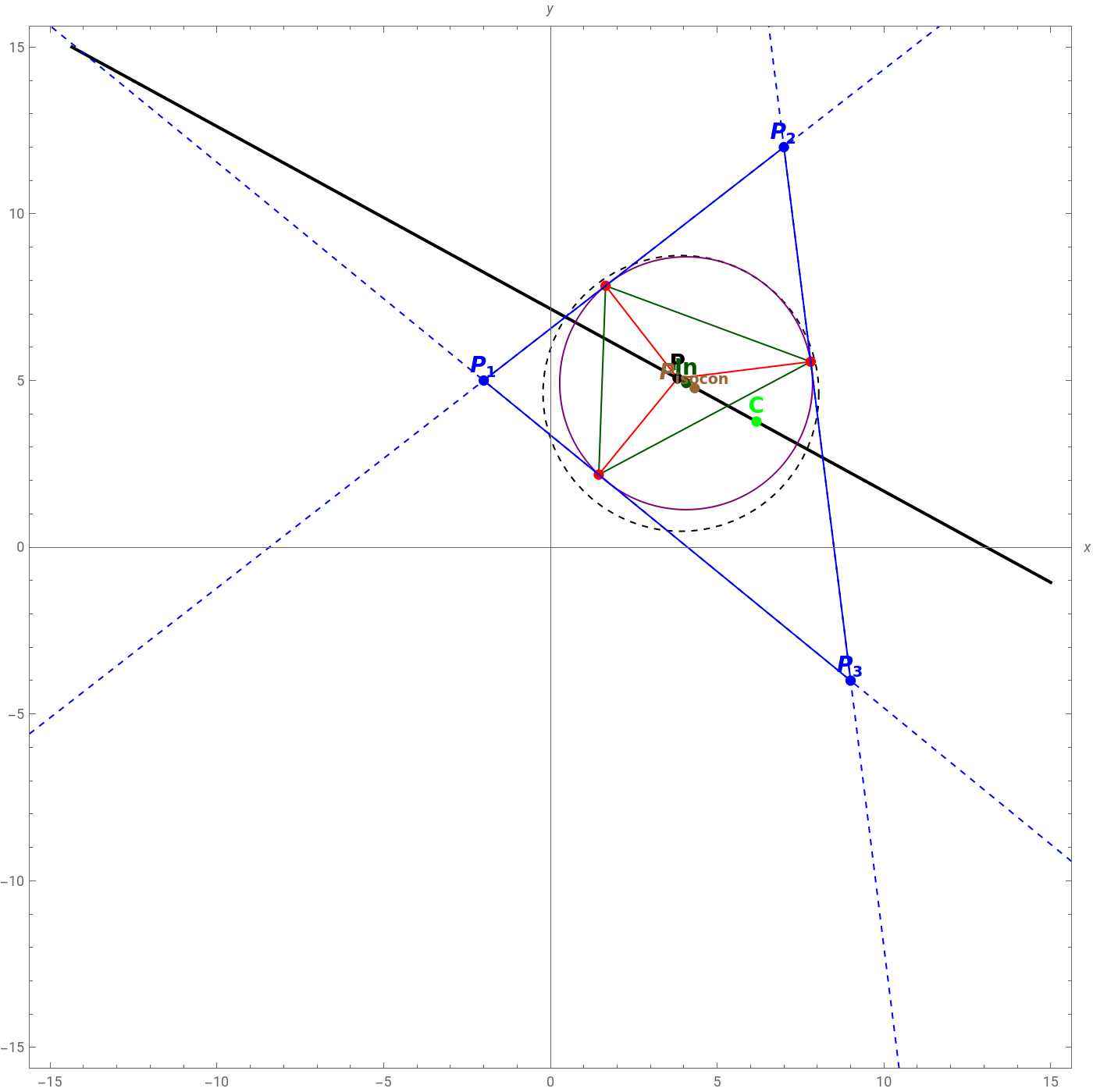
In the animation scroll manually and when the isogonal conjugate of P (in brown color), is on the line , the pedal circumference will be tangent to the 9 points circumference, fulfilling the third theorem of Fontené.
Example 2:
In[]:=
Manipulatex1=0;y1=0;x2=1;y2=0;x3=;y3=;tri={0,0},{1,0},,;α=TriangleCenter[tri,"Circumcenter"];α1=TriangleMeasurement[tri,"Circumradius"];xc=α[[1]];yc=α[[2]];Circumcenter={xc,yc};β=TriangleCenter[tri,"NinePointCenter"];xn=β[[1]];yn=β[[2]];β1=TriangleMeasurement[tri,"NinePointRadius"];γ=TriangleCenter[tri,"Incenter"];xin=γ[[1]];yin=γ[[2]];Incenter={xin,yin};m=;P={x,yin+m(x-xin)};PP1=N,N-;PP2=N,N;PP3={x,0};tri1={PP1,PP2,PP3};ξ=TriangleCenter[tri1,"Circumcenter"];xc1=ξ[[1]];yc1=ξ[[2]];ξ1=TriangleMeasurement[tri1,"Circumradius"];=N297-14930+4221",14,Bold],{x1,y1},{0,-1.2}]}],Graphics[{Blue,PointSize[0.01],Point[{x2,y2}],Text[Style["",14,Bold],{x2,y2},{0,-1.2}]}],Graphics[{Blue,PointSize[0.01],Point[{x3,y3}],Text[Style["",14,Bold],{x3,y3},{0,-1.2}]}],Graphics[{Red,PointSize[0.01],Point[PP1]}]/.xk1,Graphics[{Red,PointSize[0.01],Point[PP2]}]/.xk1,Graphics[{Red,PointSize[0.01],Point[PP3]}]/.xk1,Graphics[{Purple,Circle[{xc1,yc1},ξ1]}]/.xk1,Graphics[{Blue,TriangleConstruct[tri,"Boundary"]}],Graphics[{Brown,PointSize[0.01],Point[],Text[Style["",14,Bold],,{0,-1.2}]}]/.xk1},AxesTrue,AxesLabel{x,y},AxesOrigin{0,0},AspectRatioAutomatic,PlotRange1.5,ImageSize700],{k1,-1.5,1.5,0.00001}
3
10
7
10
3
10
7
10
yc-yin
xc-xin
9-35
2
+358
+7-10-32
+58
x10-4-7
2
+58
77+5
2
-58
+-10-32
+58
x10-4-7
2
+58
-609+42
58
+3290-2032
+58
x290-4-7
2
+58
7-203+14
58
+290-2032
+58
x290-4-7
2
+58
P
ic
2
+75629
+59358
+4x99807-1141562
+278629
+568258
+x-200132+1942152
-726629
-410558
-20-6292+44172
-37129
+27158
x10174-2032
+958
+20-29+258
x7-87+582
-829
+658
+4-1856+14729
+10058
(-1+x)x,N-873+352
+329
140+692
+2x8584+62932
-233829
-29158
-24582+20302
-130929
+9058
x70-87+582
-829
+658
+40-1856+14729
+10058
(-1+x)x;Show[{ContourPlot[mx-y-mxin+yin==0,{x,-1.5,1.5},{y,-1.5,1.5},ContourStyle->{Black,Thick}],Graphics[{Red,Line[{P,PP1}]}]/.xk1,Graphics[{Red,Line[{P,PP2}]}]/.xk1,Graphics[{Red,Line[{P,PP3}]}]/.xk1,Graphics[{Blue,Dashed,InfiniteLine[{{x1,y1},{x2,y2}}]}],Graphics[{Blue,Dashed,InfiniteLine[{{x1,y1},{x3,y3}}]}],Graphics[{Blue,Dashed,InfiniteLine[{{x2,y2},{x3,y3}}]}],Graphics[{DarkGreen,TriangleConstruct[tri1,"Boundary"]}]/.xk1,Graphics[{Black,PointSize[0.01],Point[P],Text[Style["P",14,Bold],P,{0,-1.2}]}]/.xk1,Graphics[{Black,Dashed,Circle[{xn,yn},β1]}],Graphics[{Green,PointSize[0.01],Point[Circumcenter],Text[Style["C",14,Bold],Circumcenter,{0,-1.2}]}],Graphics[{DarkGreen,PointSize[0.01],Point[Incenter],Text[Style["In",14,Bold],Incenter,{0,-1.2}]}],Graphics[{Blue,PointSize[0.01],Point[{x1,y1}],Text[Style["P
1
P
2
P
3
P
ic
P
isocon
P
ic
Out[]=
Example 3: