The stability of an orbit plays several important roles. The stability of an orbit effects the energy spent by an object to stay in orbit, whether it’s a satellite transmitting data or a spacecraft parking in the orbit. The most commonly seen model, Keplerian, applies most accurate to a spherical mass. Irregularly shaped objects, like ellipsoids or even more deformed shapes, will experience discrepancies in their gravitational fields compared to the ellipse seen in the Keplerian model. These gravitational disturbances make it difficult for objects to fall into a stable orbit around these bodies. In this computational essay, I conduct a case study of Phobos, searching for stable orbits computationally.
Introduction
Introduction
We approach the problem by calculating the gravitational field around an irregular object by taking the summation of individual gravitational fields of every within the body of Phobos. From here, we can solve the differential equation for the positions of the bodies. After creating models of orbits, we needed to find stable orbits. Two methods that are tested in my computation are the Distant Retrograde Orbits and Halo Orbits of Phobos. We model these orbits and calculate the Lyapunov exponents to determine the stability.
2-Body and 3-Body Orbital Trajectories
2-Body and 3-Body Orbital Trajectories
Importing Data
Importing Data
This computational essay performs a case study of Mars’ moon Phobos, but the same approach can be taken for any body we have data on. Through past observation, data on Phobos’ shape, mass, orbital period, etc. has already been collected. There is not, however, precise data on the mass distribution of Phobos, so for this essay, we assume it has a uniform density.
Define constants used in this simulation. We use Mars as the frame of reference setting it to the position of {0,0,0}. All constants are in SI units, with distance in meters and time in seconds.
In[]:=
G= QuantityMagnitude[UnitConvert@];massMars = QuantityMagnitude massPhobos = QuantityMagnitude periodPhobos =QuantityMagnitude *3600angularVPhobos = 2 * Pi / periodPhobosposPhobos = {0,9376000, 0};posMars= {0,0,0};
Out[]=
6.417×
23
10
Out[]=
1.072×
16
10
Out[]=
2.76×
4
10
Out[]=
0.000228
The data is imported in kilometers, so we scale Phobos up by 1000 to convert .
In[]:=
phobos = Scale[ResourceData["Phobos"],{1000,1000,1000}]
Out[]=

The imported data is a mesh region of consisting of thousands of triangles which make up the surface. For this problem, we don’t require the exact texturing of the surface of Phobos, so we coarsen the shape of Phobos for faster computations in the future. There are several approaches to this problem, but we’ve decided to take a random sample of points from within the region.
In[]:=
meshPrim = MeshPrimitives[phobos,2];
Take a random sample of 3000 points from the original mesh as a representation of the surface. Take a convex hull mesh of this surface sample, then sample div = 1000 random points within the region to represent the shape of the mass of Phobos.
In[]:=
div=1000;surfaceSample=RandomPoint[phobos,3000];ch=ConvexHullMesh[surfaceSample];internalSample=RandomPoint[ch,div];ListPointPlot3D[internalSample]
Out[]=

We assume Phobos has uniform density, so we can assign an equal mass to the 1000 points. We take the mass at each of these points as (Mass of Phobos)/(Number of Points).
In[]:=
massPhobosParticle = massPhobos / div;phobosCoM = Mean[internalSample];
Gravitational Field
Gravitational Field
The gravitational field is determined using the equation -. When we have a near spherical mass or a significant distance, we can generally solve the equation using a point mass. However, for Phobos, it is quite irregular. We instead take the sum of the gravitational field of several points within Phobos to account for the irregular shape.
a
g
G*M
2
r
The function takes the 3D Cartesian coordinates and the list representing the source of gravity as input. It returns the acceleration due to gravity of the given body as a vector at the given point.
In[]:=
irregGrav[x_,y_,z_,m_,largeBody_]:={Sum[-((G*m)(x-largeBody[[i]][[1]]))/((x-largeBody[[i]][[1]])^2+(y-largeBody[[i]][[2]])^2+(z-largeBody[[i]][[3]])^2)^(3/2),{i,Length[largeBody]}],Sum[-((G*m)(y-largeBody[[i]][[2]]))/((x-largeBody[[i]][[1]])^2+(y-largeBody[[i]][[2]])^2+(z-largeBody[[i]][[3]])^2)^(3/2),{i,Length[largeBody]}],Sum[-((G*m)(z-largeBody[[i]][[3]]))/((x-largeBody[[i]][[1]])^2+(y-largeBody[[i]][[2]])^2+(z-largeBody[[i]][[3]])^2)^(3/2),{i,Length[largeBody]}]}
This function returns the acceleration due to gravity assuming a point mass. It produces a more regular gravitational field, and it is used for further and more spherical objects used in this computational essay such as Mars.
In[]:=
regGrav[x_,y_,z_,m_,p1_,p2_,p3_]:={-((G*m)(x-p1))/((x-p1)^2+(y-p2)^2+(z-p3)^2)^(3/2),-((G*m)(y-p2))/((x-p1)^2+(y-p2)^2+(z-p3)^2)^(3/2),-((G*m)(z-p3))/((x-p1)^2+(y-p2)^2+(z-p3)^2)^(3/2)}
Modeling the positions
Modeling the positions
The two functions above give the acceleration due to gravity of an object, or the second derivative. We can solve the 2nd order ODE for the position vectors of the bodies involved in the simulation.
2-Body Simulation
2-Body Simulation
For this 2-Body simulation, we temporarily use Phobos as the reference frame, setting it at {0,0,0}.
Define the initial positions and velocities needed to solve for the position as a function of time after integrating the acceleration.
In[]:=
initPosSatellite2Bod={0,0,20000};initVelSatellite2Bod={0,5.9811577474599344`,0};initPosMars2Bod={0,0,0};initPosMars2Bod={0,0,0};
From here, we can set up our differential equation. In this case, it’s quite simple. Since the mass of the satellite is extremely small, it exerts a negligible influence on Phobos. Thus, we don’t need to worry about Phobos’ position changing. We make use of NDSolve to compute the position of the satellite given the initial conditions.
The equations describe the satellite’s acceleration, initial velocity, and initial position.
In[]:=
eqnsMotion2Body={{x1''[t],y1''[t],z1''[t]}==(irregGrav[x1,y1,z1,massPhobosParticle,internalSample]/.{x1->x1[t],y1->y1[t],z1->z1[t]}),x1[0.]==initPosSatellite2Bod[[1]],y1[0.]==initPosSatellite2Bod[[2]],z1[0.]==initPosSatellite2Bod[[3]],x1'[0.]==initVelSatellite2Bod[[1]],y1'[0.]==initVelSatellite2Bod[[2]],z1'[0.]==initVelSatellite2Bod[[3]]};
Solving generates a list of coordinates for the satellite over time, which we save as variables.
In[]:=
opTime=150000;{xFunc2Bod,yFunc2Bod,zFunc2Bod}=NDSolveValue[eqnsMotion2Body,{x1,y1,z1},{t,0.,opTime,10}];
We save the data in a table which takes the list up until a given parameter time.
In[]:=
trajectoryData2Body[time_]:=Table[{xFunc2Bod[t],yFunc2Bod[t],zFunc2Bod[t]},{t,0,time,1}];
For a better view of the orbital trajectories, we can plot all the points that the particle has passed through in the given time frame. This orbital trajectory can be seen in as an attachment.
In[]:=
Animate[Graphics3D[{Line[trajectoryData2Body[t]],phobos}],{t,0,opTime,100}]
Out[]=
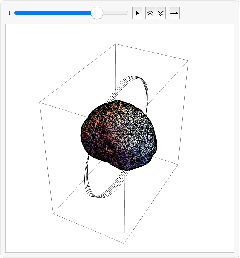
Changing the initial conditions so that the satellite starts on a different trajectory. The process is the same as above. The orbital trajectory is shown as an attachment.
We see visually that the satellite orbits around Phobos, but it isn’t unable to find a stable orbit. The satellites angle of rotation and distance from Phobos varies with time, making the satellite likely to either escape the gravitational pull of Phobos or crash into Phobos itself. Later in this computational essay, we provide an analytical method of determining the stability of an orbital trajectory using the Lyapunov exponent.
3-Body Simulation
3-Body Simulation
Defining initial conditions for a 3-Body System of Mars, Phobos, and the satellite.
We once again use the acceleration to solve for the position as a function of time. When we have three bodies, the satellite is affected by both Mars and Phobos so we sum their two gravitational fields. Like in the 2-Body calculation, the satellite has a negligible force on Mars and Phobos, so we don’t factor it into the positions of those two bodies. Additionally, Mars is approximately spherical and is at a large distance from Phobos and the satellite, so we calculate gravitational field due to Mars assuming Mars is a point mass.
Use NDSolve to solve for position as a function of time.
The orbital trajectories are shown, with purple showing Mars, green showing Phobos, and blue showing the satellite.
This visual zooms in on Phobos, as the interaction between Phobos and the satellite is difficult to see in the graphic above. Blue still tracks the satellite, while green shows Phobos. This is modeled in GIF 3.
Analyzing Orbital Stability
Analyzing Orbital Stability
Gravitational Potential Fields
Gravitational Potential Fields
The function calculates the gravitational potential at a given point (x,y,z) caused by an irregular body given as a list of points.
The function calculates the gravitational potential at a given point (x,y,z) caused by a point mass at {p1,p2,p3}. We can use this to calculate the potential when the larger body is approximately spherical or a large distance away.
Using the first potential function for the irregularly shaped Phobos, we can create a plot in 3D that shows the gravitational potential field in 3D. We use a density plot to show the gravitational potential in 3D space.
We can also plot the difference between potentials of Phobos’ potential when considered as an irregularly shaped object and when considered as a perfectly spherical object with the same mass as Phobos. This model shows the discrepancies found when comparing an irregularly shaped object and a perfect sphere. In the graphic below, the purple represents points where the magnitude of Phobos’s gravitational potential is greater than that of a point with the same mass as Phobos. The magenta color is the opposite.
Lagrangian Points
Lagrangian Points
In this contour plot of the potentials, the mass of Phobos is increased by a scale of 10 million for the sake of visualization purposes.
It is important to note points where the gravitational potential doesn’t change. An object placed within this field can be balanced at points where the potential doesn’t change. We notice one such point in between the two planetary bodies. However, when we set the objects into a rotational motion with Phobos orbiting Mars, we observe five such points in which there is no change in the gravitational potential. These are the Lagrangian points, which are relatively stable positions in an orbit for spacecrafts to orbit without burning too much energy.
Define variables needed for these computations.
The previous graph plotted the gravitational field caused by Mars and Phobos in a still reference frame. However, in order to see the Lagrangian points, there needs to be rotational motion. To keep the graph stationary however, we’ve instead decided to model the graph using a rotational reference frame. The reference frame turns at the same rate as Phobos’ angular velocity, so Mars and Phobos appear stationary in the new reference frame.
Define the function that describes potential given a point in a rotational reference frame.
A plot where potential is plotted on the Z-axis helps for visualization. We can visualize objects rolling from points with higher potential to points with lower potential. A corresponding contour plot is also included.
We reproduce the same images as above, but this time we exaggerate Phobos’ mass by a factor of 10^7 for the sake of visualization.
Using this function, we produce two plots that show the presence of the Lagrange points. The first, a contour plot, exhibits five areas in which the contours don’t cross over. These are the Lagrange points, in which there exists an area where the change in gravitational potential is 0.
This second graph, which plots gravitational potential in the Z direction, makes the visualization even more simple. The 5 Lagrange points lie at the points when the plot maps out a flat surface. These are the points at which a ball would balance if placed perfectly – similarly, spacecrafts can balance gravitational forces at these points when orbiting.
We know that -∇U = F. The 5 Lagrange points can be found by taking points where the gradient of the potential function is 0. Connecting this, we can confirm that gravitational force at the Lagrange points should be balanced in all directions. Let us return to the unscaled version of the potential function to find solutions to -∇U = 0.
Solve for {x,y} such that the partial derivative of the potential derivative with respect to x and y are both 0.
After taking real solutions, we end up with this list of the five Lagrangian points:
This is the gravitational field zoomed in to focus on L2. The satellite has less than a kilometer of distance to work with in terms of staying within the Lagrangian point, which makes the halo orbit of Phobos significantly more difficult to find.
We plot the gradient of the 2D potential function on the plane Z = 0 at the L2 point that we found in the above calculation
Halo Orbits
Halo Orbits
We can see from the graph above the advantage of the Lagrange point. Forces from the left and right will keep the satellite centered in the tangential direction. Balanced forces in the radial direction minimizes the need for fuel thrusters. Let us attempt to model a halo orbit.
We now move to mapping the potential function in 3D.
We take the gradient of the function above.
The function returns the Coriolis force given the velocity.
Theoretically, the halo motion is caused by the gravitational forces, the centrifugal force, and the Coriolis force. However, Phobos is extremely small, so instead of the above calculations, we use a dimensionless system to model the trajectories.
The originally complicated system including high order differential equations was simplified by Farquhar-Kamel. (Breakwell & Brown, 1979).
The originally complicated system including high order differential equations was simplified by Farquhar-Kamel. (Breakwell & Brown, 1979).
We set up the system of differential equations.
Solve the differential equation system, then plot the trajectories.
We can model many different set ups by changing the initial conditions.
Projections on the x-y plane
Projections on the y-z plane
Lyapunov Exponent
Lyapunov Exponent
The Jacobian is a linearization to get the first order derivative.
Solves the differential equation.
We define vector operations used later on like projection and the Gram-Schmidt process;
Calculating Lyapunov for Halo Orbits
Calculating Lyapunov for Halo Orbits
We follow Kathleen Howell’s method to find the Lyapunov for halo orbits (Howell)
We convert the 2nd order ODEs to 1st order.
We integrate over a combined system of differential equations given in Sandri’s paper. The code outputs an estimate for the Lyapunov exponent.
As we continue to apply the process above, we plot the limit as number of steps goes to infinity.
Calculating Lyapunov for Distant Retrograde Orbits
Calculating Lyapunov for Distant Retrograde Orbits
We can apply the same algorithm to the distant retrograde orbits that we modeled early on in the computational essay. First, we find the Lyapunov function of a 2-Body system in which we assume that Phobos is a point mass.
Now, we test it while factoring in the fact that Phobos is irregularly shaped, and we observe that it is higher than the calculated Lyapunov exponent for a point mass Phobos.
Conclusion
Conclusion
We model the gravitational field and gravitational potential to help model the motions of a satellite around an irregularly shaped celestial body like Phobos. While modeling orbits in the 2-Body and 3-Body system, we found that while orbits exhibited some semblance of a regular orbit early on, they eventually became chaotic. In light of this, we attempted to search for and model more stable Distant Retrograde Orbits or Halo orbits by finding the Lagrangian points. We analytically calculate the stability of these orbits by using Lyapunov exponents and found that the orbits generally were classified as moderately chaotic.
Future Directions
Future Directions
A large assumption made was that Phobos, or any other body we could’ve used, had a uniform density. Depending on the body we’re studying, this could have a varied degree of impact. For example, the Moon’s density is skewed heavily despite having a rather spherical shape, which prevents the presence of stable orbits. Due to time constraints, we’ve also assumed modeled our halo orbits assuming Phobos to be a point mass, as the function that accounts for the mass irregularities was unable to run properly. Past orbits, we can use the same data to model maneuvers where spacecrafts utilize irregularly shaped objects for gravitational assists, deflections, or temporary parking.
References
References
◼
Benettin, G., Galgani, L., Giorgilli, A. et al. Lyapunov Characteristic Exponents for smooth dynamical systems and for hamiltonian systems; a method for computing all of them. Part 1: Theory. Meccanica 15, 9–20 (1980). https://doi.org/10.1007/BF02128236
◼
Breakwell, J.V., Brown, J.V. The ‘Halo’ family of 3-dimensional periodic orbits in the Earth-Moon restricted 3-body problem. Celestial Mechanics 20, 389–404 (1979). https://doi.org/10.1007/BF01230405
◼
Connor Howell, K. Three-dimensional, periodic, ‘halo’ orbits. Celestial Mechanics 32, 53–71 (1984). https://doi.org/10.1007/BF01358403
◼
Sandri, M. (n.d.). Numerical calculation of lyapunov exponents. https://venturi.soe.ucsc.edu/sites/default/files/Numerical_Calculation_of_Lyapunov_Exponents.pdf
Acknowledgements
Acknowledgements
I sincerely appreciate my mentor Shenghui Yang for guiding me through this process and making each class a ton of fun. I also want to extend a special thanks to Gregory Roudenko for peer reviewing my computational essay and giving advice throughout the process. Finally, I thank my peers in this program for brightening the atmosphere and keeping me company.
CITE THIS NOTEBOOK
CITE THIS NOTEBOOK
Modeling and evaluating orbital trajectories of irregular objects such as phobos
by Richard Fan
Wolfram Community, STAFF PICKS, July 11, 2025
https://community.wolfram.com/groups/-/m/t/3502464
by Richard Fan
Wolfram Community, STAFF PICKS, July 11, 2025
https://community.wolfram.com/groups/-/m/t/3502464