Classical Marcus Equation for Photo-induced Electron Transfer Calculator: “CME-Calc” Version-1.3, 25-02-2020 “Introduction to Photo-induced Electron Transfer in Mathematica-V6”

Abstract

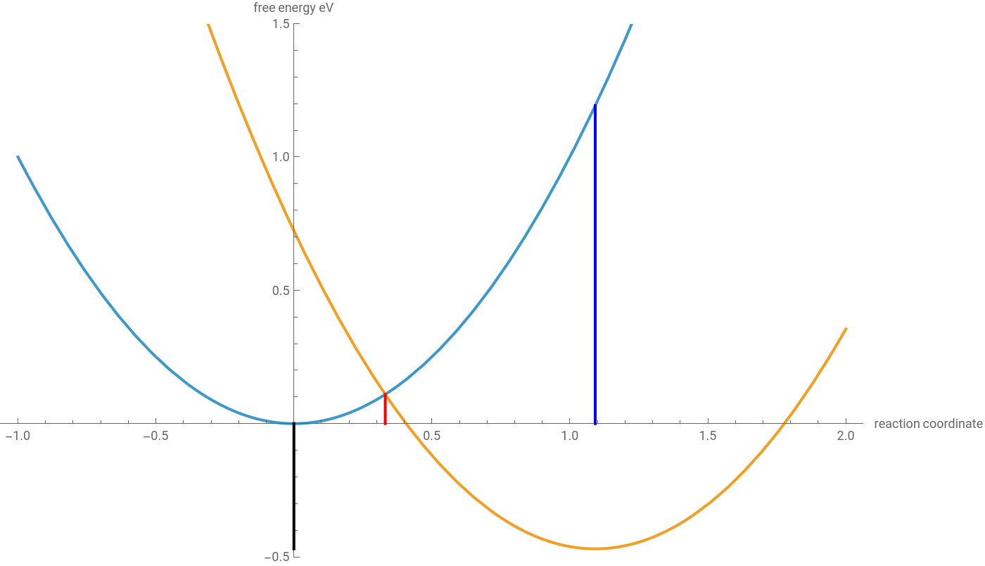
With this Calculator you can use the Classical Marcus Equation to calculate and manipulate the rate of electron transfer (charge separation) by using “molecular parameters” such as redox data, center to center distance, ionic radii, electronic coupling, internal reorganization energy, solvent reorganization energy, dielectric constants, refractive index. Driving force, total reorganization energy and barrier to electron transfer (and the pre-exponential factor) are used and calculated separately. The outcome is visualized with intersecting parabola, with driving force (black), barrier (in red) and total reorganization energy (in blue) as vertical lines. The starting data (molecular parameters) comes from C60[11]DMA in benzonitrile solvent, published in 1996 (see below). For neutral starting donor and acceptor the Coulomb Correction (z) is 1, for a charge shift reaction it is 0, for charged initial reactants it is -1. (see top right manipulator). With the other top four manipulators you can scale the graph. Above all manipulators, the standard starting values are given together with units. The slides in the graph-box are just for demonstration (data is not calculated/updated). With the top right + sign you can bookmark input data to recall later. This projects is best viewed at 100 %. The second part is some clarification of the equations and constants, the driving force and the Marcus Bell-shaped curve. Some examples using literature data/test data are given.

Manipulate

Out[]=

-0.469683

Gibbs Free Energy for electron transfer, (eV):

1.19256

Total Reorganization energy, (eV):

0.109543

Barrier to electron transfer, (eV):

5.62409×

Rate of electron transfer,



-1

:

4.19524×

Pre-exponential factor,

opt



-1

:

expansion left x-axis), 1

expansion right x-axis), 2

expansion low y-axis, 0.5

0.5

expansion high y-axis, 1.5

1.5

Coulomb Correction, 1

Eox, (eV), 0.71

0.71

Ered, (eV), -0.57

-0.57

Eoo, (eV), 1.76

1.76

eps, epsilon, 25.2

25.2

Rc, distance (A), 18

epsEC, 37.5

37.5

Ran, anion radius (A), 5.6

5.6

Rcat, cation radius (A), 3.7

3.7

Li (eV), 0.3

0.3

n, 1.528

1.528

V, coupling (cm^-1), 43

T, temperature, 295

294.8

y Driving force

-0.469683

x Reorganization

1.19256

Gibbs free energy (eV) -0.469683

reorganization energy (eV) 1.19256

energy of activation (eV) 0.110

rate (s^-1) 5.62409×

Caption

By using 8 molecular input parameters and 4 general input parameters, we can calculate the Gibbs Free energy of electron transfer (DeltaG), the barrier (Ea), the total reorganization energy (LambdaT) as well as the rate of the charge separation (Ket). The pre-exponential factor is the rate that can be obtained if no barrier is present (kopt). By using the sliders of the manipulators (or changing the values manually in the box), we can see the effects of all individual parameters on the rates and thermodynamic quantities. The blue curve is the initial reactants (locally excited state), the yellow curve is the final product (after charge separation). The black, red and blue vertical lines represent the magnitude of the driving force , barrier and total reorganization energy. Eox and Ered are the redox data of the donor and acceptor (in same solvent with dielectric constant (= epsEC) vs the same reference electrode ), Rc = center to center distance, Ran and Rcat are the ionic radii, V = electronic coupling, Li = internal reorganization energy, dielectric constants (eps) , refractive index (n). Eoo = singlet state energy (or triplet state energy) of the system.

Equations and Data

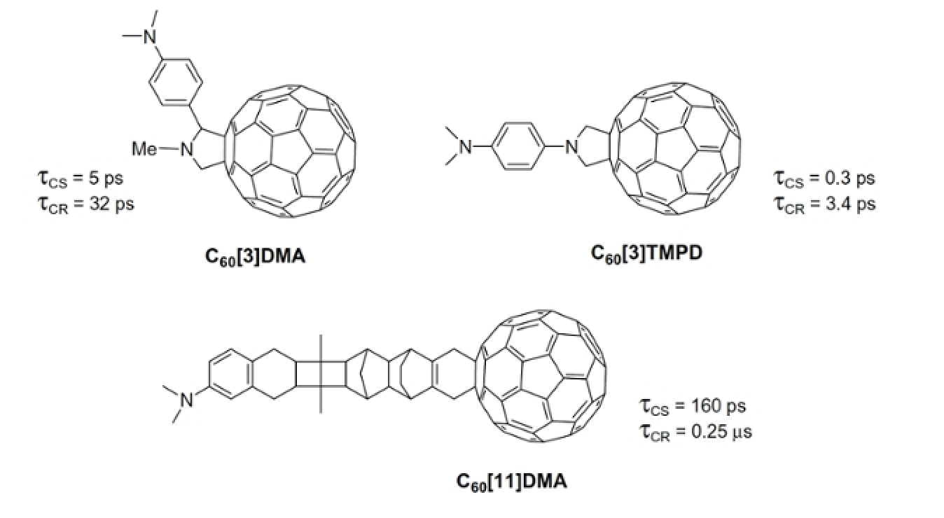
The equations that are used in this project are given below obtained from the actual code. They can be found in the Mathematica (.nb) file which is available next to the CDF file.

The equations are also given in the regular form:

(r = average ionic radius)

These general equations, and background information on the theory of electron transfer, are described in:https://www.researchgate.net/publication/225188430_Introduction _to _Electron _TransferData (see below for test data) from the following papers is used:JOC 1996:https://pubs.acs.org/doi/abs/10.1021/jo960678qJACS 1995:https://pubs.acs.org/doi/abs/10.1021/ja00119a025My PhD thesis (containing all data, and corrected data, from the two papers above).http://dare.uva.nl/document/17261JACS 1987 (Oevering):https://pubs.acs.org/doi/abs/10.1021/ja00245a014

These three compounds are described in the JACS 95 and JOC 96 papers.Transfer times in benzonitrile for C60[3]DMA and C60[11]DMA. Transfer times in toluene for C60[3]TMPD.New (fast) rates for top two compounds are reported in https://www.researchgate.net/publication/256238490_Energy _and _Electron _Transfer _in _Photo-_and _Electro-Active_Fullerene _Dyads(see below for some test data).

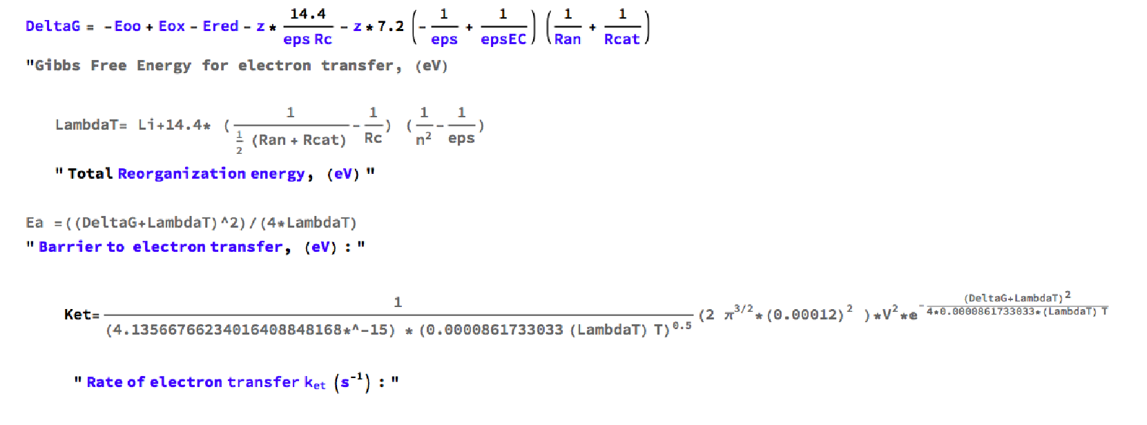
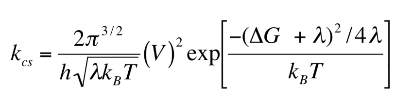
Constants

For clarity and convenience the constants are described here, within their Mathematica context (in text format). You can copy and paste it as code into Mathematica. The constants can be found in many other places. It has to be noted that the refractive indices and dielectric constants of solvents have to be looked up from other sources.

Driving Force

We can plot the driving force as a function of distance, and change the dielectric constant of the medium with the slider. In a polar medium the Gibbs free energy change is not very sensitive to the distance between donor and acceptor, but in a non-polar medium the distance has a much larger effect on the driving force (see also JACS 1987), (change of eps).(Click on small + sign before number to change manually).

If we plot the driving force as function of dielectric constant we can determine which conditions make charge separation feasible.

This graph shows the Delta G as function of epsilon of the solvent. We can determine which polarity (eps) we need to get PET. We need an epsilon higher than ~8 to quench the triplet state of C60[11]DMA.
(see JOC 96, Table 3 or test data below). Check that this graph flips sign if Rc is much smaller than the sum of Ran and Rcat divided by two (see Notes).

Marcus Bell-shaped Curve

Perhaps the most well known graph of the Marcus Theory of Electron Transfer is the one that shows the effect of the Inverted Region. The rate of electron transfer as function of the Gibbs Free Energy change. The “left” side of this graph shows that the rate goes down if the driving force goes up further, beyond the Optimal Region (top of the curve).
So what is the effect of changing the total reorganization energy (Lambda) or going to 77 Kelvin?? (Click on small + sign before number to change manually).

Snapshots

Notes

Authoring information

After three decades of trying to understand, applying and teaching about the Marcus Theory of Electron Transfer,
it was time for the next step: an interactive form of this Nobel price winning theory is now available to all!!
(note that an interactive FCWD factor is still missing!).
It seems that quite a few people (~10 000) have been interested in my ‘Introduction to Electron Transfer”,
so I spend some time to make this material more accessible and hopefully easy to apply to real research cases.

A semi-classical version for charge recombination, similar to this notebook, is in the planning...

Challenges:
Can we use the Marcus model for ultrafast charge formation into delocalized states?
(use larger anionic radius??).
http://science.sciencemag.org/content/343/6170/512

Can we explain the recent data of Arnaut et al. with the Marcus model?
(data seems good, interpretation is questionable, see figure 5b and Marcus Bell curve T info above.
Figure 5a seems like two separate non-linked data sets. Check ref. 15, note about chlorinated solvents ).
https://www.nature.com/articles/s41467-018-05267-5