ABSTRACT (original article): In linear perturbation theory, the ringdown of a gravitational wave (GW) signal is described by a linear combination of quasinormal modes (QNMs). Detecting QNMs from GW signals is a promising way to test GR, central to the developing field of black-hole spectroscopy. More robust black-hole spectroscopy tests could also consider the ringdown amplitude-phase consistency. That requires an accurate understanding of the excitation and stability of the QNM expansion coefficients. In this paper, we investigate the robustness of the extracted m=2 QNM coefficients obtained from a high-accuracy numerical relativity waveform. We explore a framework to assess the robustness of QNM coefficients. Within this framework, we not only consider the traditional criterion related to the constancy of a QNM’s expansion coefficients over a window in time, but also emphasize the importance of consistency among fitting models. In addition, we implement an iterative greedy approach within which we fix certain QNM coefficients. We apply this approach to linear fitting, and to nonlinear fitting where the properties of the remnant black hole are treated as unknown variables. We find that the robustness of overtone coefficients is enhanced by our greedy approach, particularly for the (2, 2, 2, +) overtone. Based on our robustness criteria applied to the m=2 signal modes, we find the (2~4, 2, 0, +) and (2, 2, 1~2, +) modes are robust, while the (3, 2, 1, +) subdominant mode is only marginally robust. After we subtract the contributions of the (2~4, 2, 0, +) and (2~3, 2, 1, +) QNMs from signal mode (4, 2), we also find evidence for the quadratic QNM (2, 1, 0, +)×(2, 1, 0, +). CITATION (original article): L. Gao, G. B. Cook, et al. (2025), The robustness of extracting quasinormal mode information from black hole merger simulations, arXiv:2502.15921 (Submitted to Physical Review D). https://doi.org/10.48550/arXiv.2502.15921
GitHub (with data files): https://github.com/cookgb/KerrRingdown
GitHub (with data files): https://github.com/cookgb/KerrRingdown
Related articles
Related articles
The ringdown fitting methods used in the KerrRingdown Paclet were developed in the following paper:
G. B. Cook, Aspects of multimode Kerr ringdown fitting, Phys. Rev. D, vol. 102, no. 2, p. 024 027, 2020. doi: 10.1103/PhysRevD.102.024027. arXiv: 2004.08347 [gr-qc]. https://doi.org/10.1103/PhysRevD.102.024027
G. B. Cook, Aspects of multimode Kerr ringdown fitting, Phys. Rev. D, vol. 102, no. 2, p. 024 027, 2020. doi: 10.1103/PhysRevD.102.024027. arXiv: 2004.08347 [gr-qc]. https://doi.org/10.1103/PhysRevD.102.024027
This results in this paper are obtained through the following version of Paclet:
G. B. Cook and L. Gao, KerrRingdown, version v1.0.0, 2025. doi: 10.5281/ zenodo.14804284. Available: https://doi.org/10.5281/zenodo.14804284.
G. B. Cook and L. Gao, KerrRingdown, version v1.0.0, 2025. doi: 10.5281/ zenodo.14804284. Available: https://doi.org/10.5281/zenodo.14804284.
L. Gao, G. B. Cook, et al., The robustness of extracting the quasinormal modes information from black hole merger simulation, (2025), arXiv:2502.15921 [gr-qc]. (Submitted to Physical Review D). https://doi.org/10.48550/arXiv.2502.15921
Two new features ( Greedy fitting and quadratic modes ) described in the paper above are introduced to the version v1.1.0 of the paclet:
G. B. Cook and L. Gao, KerrRingdown: Greedy fitting and quadratic modes, version v1.1.0, 2025. doi: 10.5281/zenodo.14804284. Available: https://doi.org/10.5281/zenodo.14861548.
G. B. Cook and L. Gao, KerrRingdown: Greedy fitting and quadratic modes, version v1.1.0, 2025. doi: 10.5281/zenodo.14804284. Available: https://doi.org/10.5281/zenodo.14861548.
Other papers related with the KerrRingdown Paclet:
L. Magaa Zertuche, L. Gao, E. Finch, and G. B. Cook, Multimode ringdown modelling with qnmfits and KerrRingdown, (2025), arXiv:2502.03155 [gr-qc]. https://doi.org/10.48550/arXiv.2502.03155
L. Maga
n
Introduction
Introduction
The final stage of binary black hole (BBH) coalescence, known as the ringdown, results in the formation of a remnant Kerr black hole. According to linear perturbation theory in general relativity (GR), a certain period of the ringdown gravitational-wave (GW) signal emitted by the perturbed Kerr black hole can be described as a superposition of quasinormal modes (QNMs). In GR, the frequencies of these QNMs depend only on the mass and spin of the remnant black hole, embodying the black hole no-hair theorem. This leads to the proposal of testing GR by measuring QNMs in observed ringdown signals, known as black-hole spectroscopy. Meanwhile, the excitation of these QNMs during the ringdown depends on the properties of the progenitor BBH system. A deeper theoretical understanding of QNM excitation patterns is valuable for various applications, such as constructing surrogate waveform models and more robust black hole spectroscopy tests. One crucial step in this direction is performing ringdown fitting to extract QNM coefficients from numerical relativity (NR) waveforms.
The Paclet provides an extensible structure for analyzing gravitational-wave ringdown signals by fitting a signal to the Quasinormal Modes (QNMs) of the Kerr geometry. The Paclet currently provides routines to read in gravitational-wave data sets from the SXS collaboration, but support for other collections of gravitational-wave data sets can be easily added. An extensive set of tabulated spin-weight -2 QNMs, available from the Zenodo repository https://doi.org/10.5281/zenodo.14024959, can be used as the basis for the ringdown fitting.
In this notebook, we give the most basic examples to illustrate the functionality of the KerrRingdown` Paclet and the physics behind it. The more advanced usage of this Paclet can be found in the detailed built-in documentation and the papers.
KerrRingdown`
In this notebook, we give the most basic examples to illustrate the functionality of the KerrRingdown` Paclet and the physics behind it. The more advanced usage of this Paclet can be found in the detailed built-in documentation and the papers.
Load in KerrRingdown
Load in KerrRingdown
In[]:=
PacletDir="/Users/gaoleda/Downloads/KerrRingdown";
In[]:=
PacletDirectoryLoad[PacletDir]
Out[]=
{/Users/gaoleda/Downloads/KerrRingdown}
In[]:=
Needs["PacletTools`"]
In[]:=
PacletInstall["/Users/gaoleda/Downloads/KerrRingdown/KerrRingdown/build/KerrRingdown-1.1.0.paclet"]
Out[]=
PacletObject
In[]:=
Needs["KerrRingdown`"]
Read in a NR waveform and its waveform properties
Read in a NR waveform and its waveform properties
The gravitational-wave signal used for further analysis is simulated by using numerical relativity (NR) to evolve Einstein’s equations. In this notebook, the gravitational-wave information extracted from NR is represented by the gravitational strain . The gravitational-wave signal is represented as a set of spin-weight -2 spherical harmonic mode functions (t) via =(t)(θ,ϕ).The function ReadWaveforms reads in gravitational-wave signals from NR simulations and provides the signal data in the form of a set of harmonic-mode time series data (t) . The waveform we read in here is obtained from the public catalog: the Ext-CCE Waveform Database https://data.black-holes.org/waveforms/extcce_catalog.html. The waveform provided here is the dataset named SXS:BBH_ExtCCE:0001. It has been post-processed with the following procedures. First, the waveform is read in through the public Python module scri https://github.com/moble/scri. Second, the waveform is transformed to the superrest frame through the map_to_superrest_frame method in scri. The superrest frame is the correct frame in which the quasinormal modes (QNMs) are derived and computed. Finally, we have saved the waveform as an HDF file ready for reading in through ReadWaveforms. The HDF file provided here is a simplified version with only spherical harmonic modes (2, 2), (3, 2), and (4, 2) for demonstration.
h=-i
h
+
h
×
h
NR
C
ℓm
h
NR
∑
ℓm
C
ℓm
-2
Y
ℓm
C
ℓm
In[]:=
ReadWaveforms["/Users/gaoleda/Downloads/KerrRingdown",{{2,2}},T0-4.844303644560568,DataTypeSXSCCE,WaveformTypeMetric,SXSRNext292,FrameTypeCoM,DataRangeAll,SuperrestTrue]
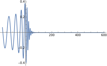
We have plotted the real part of the (l=2, m=2) spherical harmonic mode (t) below as a function of (retarded) time. The zero of time is set to be the peak amplitude of the signal. Analysis of the ringdown signal usually starts after t=0.
C
22
In[]:=
ListLinePlot[PlotReClm[2,2],PlotRangeAll]
Out[]=
The properties of the remnant black hole after binary black hole coalescence are the mass and spin. In the NR simulation, these parameters are given as the remnant mass ratio, the remnant dimensionless spin, and the remnant velocity. In this example, the remnant mass ratio δ = 0.9516, the dimensionless spin vector is {2.1×, -1.2×,0.686}. The remnant velocity is 0 because the waveform has been transformed to the superrest frame. When we perform ringdown fitting, we only focus on the first two parameters stored in BHProperties, which are the mass ratio and the magnitude of the dimensionless spin. The final two properties are the orientation angles (θ, ϕ ) of the spin vector which are not relevant since the spin vector has been rotated so that it is almost entirely in the z direction.
-11
10
-11
10
In[]:=
BHProperties=SXSFinalProperties[0.9516192579323307,2.053834297453027*10^(-11),-1.163918672685337*10^(-11),0.6864419212995438,0,0,0]
Out[]=
{0.951619,0.686442,3.43905×,-0.515578}
-11
10
Read in the QNM data
Read in the QNM data
The ringdown signal can be modeled as a superposition of the quasinormal modes (QNMs). To read in the information of the QNMs, we set the QNM data directory through HDF5QNMDir.
In[]:=
HDF5QNMDir["KerrRingdown/"]
Out[]=
KerrRingdown/
The data files in the specified directory are named , where is a 2-digit integer representing the overtone associated with all of the data stored in the file. These QNM data sets were computed using the publicly available suite of Paclets based on the approach developed by Cook and Zalutskiy (2014). The full set of data files can be downloaded from the Zenodo repository https://doi.org/10.5281/zenodo.14024959.
KerrQNMTable_nn.h5
nn
KerrModes`
The QNM data files contain the QNM frequency (a), the angular separation constant (), and the spheroidal expansion coefficients ℓm() at specific values of , where is the magnitude of the dimensionless spin. Cubic interpolation is used to obtain the data at any required value of in the range .
ω
ℓmn
-2
A
ℓm
aω
ℓmn
-2
ℓ
aω
ℓmn
a
a
a
0≤a≤1
A small subset of the compete set of data files are contained within the KerrRindown` Paclet. This data can be accessed by setting the directory to .
"KerrRingdown/"
Linear Fitting of the ringdown signal
Linear Fitting of the ringdown signal
With linear fitting, we treat the remnant mass and spin as known parameters. We only fit for the QNM expansion coefficients, which correspond to the excitations of different QNMs in the ringdown signal.
The fitting function is a linear combination of QNMs given by =, where each is an individual QNM and is the QNM expansion coefficient.
ψ
fit
ψ
fit
∑
k
C
k
ψ
k
ψ
k
C
k
Fitting is accomplished through extremizing the overlap function ρ defined by the inner product between the fitting function and the NR waveform =,where the inner products are evaluated by .The OverlapFit function within paclet is the key function for performing ringdown fitting.
ψ
fit
h
NR
2
ρ
2
〈|〉
ψ
fit
h
NR
〈|〉〈|〉
h
NR
h
NR
ψ
fit
ψ
fit
〈|〉=∮(t,Ω)(t,Ω)Ωt
ψ
1
ψ
2
t
e
∫
t
i
*
ψ
1
ψ
2
KerrRingdown
By setting the options for OverlapFit, we set the initial fitting time to vary from 0 to 50, and the end of fitting time to be a late time 90.
t
i
t
e
In[]:=
SetOptions[OverlapFit,T0TimeIndex[0],TFinalTimeIndex[50],TEndTimeIndex[90]]
Out[]=
{FitTimeStrideFalse,FixedModesGreedyFalse,FullMismatchFalse,NLmodesListFalse,PhaseChoiceSL-C,RescaleModesFalse,RestrictToSimulationSubspaceFalse,ReturnSingularValuesFalse,SVDWorkingPrecisionMachinePrecision,T02289,TEnd3441,TFinal2929,Tolerance0,UseLeastSquaresFalse}
In this example, we fit the QNMs {{2, 2, 0,+}, {3, 2, 0,+}} to the spherical harmonic modes (t) for initial fitting times :
C
22
0≤≤50
t
i
In[]:=
overlapFitResult=OverlapFit[BHProperties,{{2,2}},{{2,2,0},{3,2,0}},{}];
The overlap ρ is the second element of the OverlapFit output. We can plot the mismatch ℳ=1-ρ as a function of the initial fitting time.
In[]:=
t=overlapFitResult[[1]];ρ=overlapFitResult[[2]];ListLogPlot[Transpose[{t,1-ρ}],AxesLabel{"t","ℳ"},JoinedTrue]
Out[]=
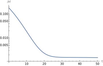
The mismatch is a quantity related to the fitting quality. A lower mismatch closer to 0 usually indicates a better fit, although overfitting can happen when too many QNMs are introduced in the fitting. For this fitting case, we can see the mismatch is low after >=25. It indicates that the ringdown signal (t) can be well-modeled by the combination of QNMs {2, 2, 0,+} and {3, 2, 0,+} after >=25.
t
i
C
22
t
i
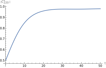
In addition to the mismatch, we can analyze the QNM coefficients obtained from fitting at each . The QNM coefficients are complex numbers, but it is more convenient to analyze their amplitudes and phases. Here we use the function FitAmplitudesTable to create a table of the amplitudes and phases with their uncertainties for all QNMs at =30.
t
i
t
i
In[]:=
FitAmplitudesTable[overlapFitResult,30.0]
Out[]=
Mode | Amplitude | Phase/π | σ(Amp) | σ(Phase)/π |
{2, 2, 0}+ | 0.978991 | -0.386494 | 0.000234098 | 0.0000761149 |
{3, 2, 0}+ | 0.045197 | -0.863233 | 0.000266136 | 0.00187433 |
We can also plot the amplitude and phase of for QNM {2, 2, 0,+}. We find that both the amplitude and phase become stabilized for >=25, which indicates a robust fitting for that time period.
+
C
220
t
i
In[]:=
t=overlapFitResult[[1]];C220=OverlapSequenceCoefPlus[overlapFitResult,{2,2,0}];
In[]:=
ListLinePlotTranspose[{t,Abs[C220]}],AxesLabel"t",""
+
C
220
Out[]=
Nonlinear Fitting to the ringdown signal
Nonlinear Fitting to the ringdown signal
Here, we use RemnantParameterSeach to calculate the OverlapFit at each grid point in the parameter space:
We can use RemnantParameterSpaceMaxOverlap to search the optimized mismatch and remnant parameters at each time based on the results obtained from RemnantParameterSearch. More accurate results can usually be obtained with this finer search.
CITE THIS NOTEBOOK
CITE THIS NOTEBOOK
The robustness of extracting quasinormal mode information from black hole merger simulations
by Leda Gao, Gregory B. Cook, et al.
Wolfram Community, STAFF PICKS, April 30, 2025
https://community.wolfram.com/groups/-/m/t/3452947
by Leda Gao, Gregory B. Cook, et al.
Wolfram Community, STAFF PICKS, April 30, 2025
https://community.wolfram.com/groups/-/m/t/3452947