Ternary Batch Rectification
Authors: Housam Binous and Ahmed Bellagi
Ternary Batch Rectification
Authors: Housam Binous and Ahmed Bellagi
Authors: Housam Binous and Ahmed Bellagi
Consider a ternary mixture composed of 30 mole% benzene, 30 mole% toluene, and 40 mole%-xylene. This mixture, which obeys Raoult’s law, is fed to the still of a batch distillation rectifier operating at . Here, the batch rectification begins with total reflux to obtain a steady state, and the distillate is withdrawn after that point. Stages and condenser holdups are assumed constant, equal to 1 and 7.5, respectively.
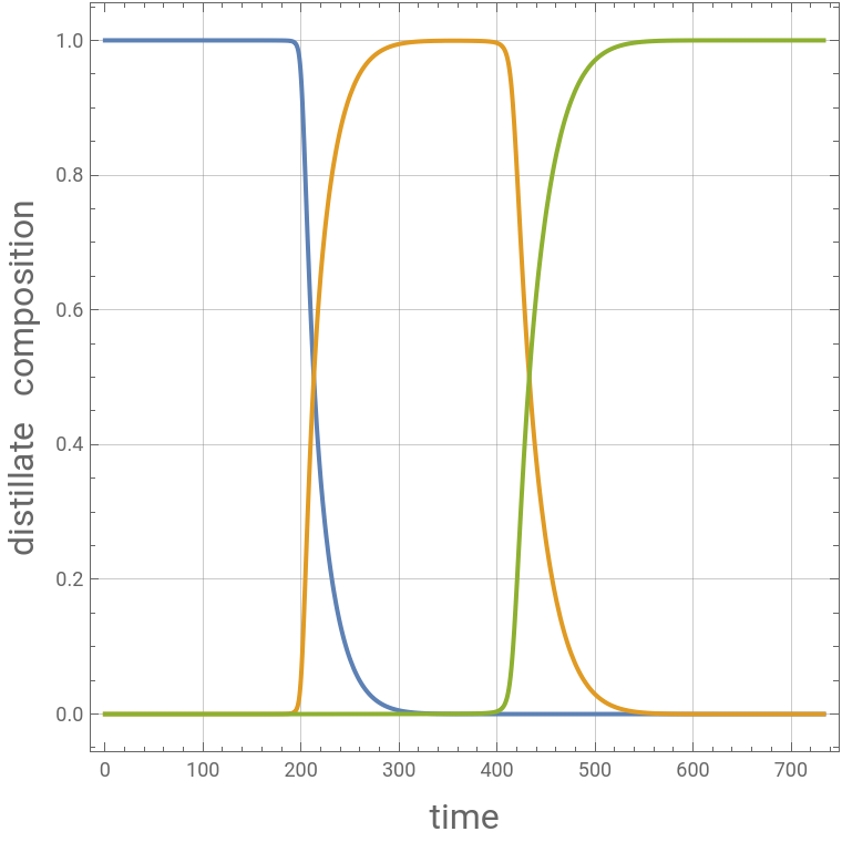
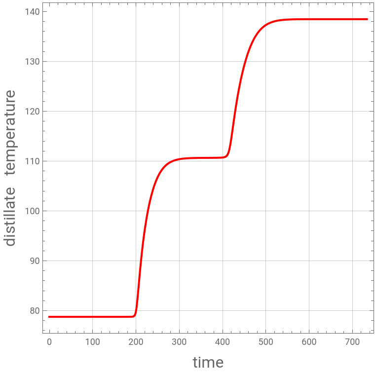
Based on the CMO (constant molal overflow) assumption, we plot the composition (curves in blue, yellow, and green for benzene, toluene, and-xylene, respectively) and the temperature of the distillate versus time, for a boil-up rate of . The values of the reflux ratio and the number of stages are chosen equal to 10 and 15, respectively . This separation is perfect when and are large. It is clear that one can collect a high-purity cut every time the distillate temperature reaches one of the plateaus .
On the other hand, for low values of the reflux ratio and number of plateaus, the separation is sloppy .
Consider a ternary mixture composed of 30 mole% benzene, 30 mole% toluene, and 40 mole%
p
P=101.325kPa
Based on the CMO (constant molal overflow) assumption, we plot the composition (curves in blue, yellow, and green for benzene, toluene, and
p
V=15
R
N
R
N
On the other hand, for low values of the reflux ratio and number of plateaus, the separation is sloppy .
For more information, see:
M. F. Doherty and M. F. Malone, Conceptual Design of Distillation Systems, New York: McGraw-Hill, 2001.
For more information, see:
M. F. Doherty and M. F. Malone, Conceptual Design of Distillation Systems, New York: McGraw-Hill, 2001.
Modified Antoine Constants
In[]:=
A1=169.65;B1=-10314.8;C1=0.;D1=-23.5895;E1=;F1=2.;A2=76.4511;B2=-6995.;C2=0.;D2=-9.1635;E2=;F2=2.;A3=91.2505;B3=-8121.25;C3=0.;D3=-11.3188;E3=;F3=2.;
2.09442
5
10
6.225
6
10
7.30555
6
10
Vapor pressure versus temperature for Benzene (component 1), Toluene (component 2), p-Xylene (component 3)
In[]:=
Psat1[i_][t_]:=/.TT[i][t];Psat2[i_][t_]:=/.TT[i][t];Psat3[i_][t_]:=/.TT[i][t];
E1+A1+D1Log[T]+
F1
T
B1
C1+T
E2+A2+D2Log[T]+
F2
T
B2
C2+T
E3+A3+D3Log[T]+
F3
T
B3
C3+T
Initial feed composition: 30 mole% benzene, 30 mole% toluene, and 40 mole% -xylene
p
In[]:=
Xf1=0.3;Xf2=0.3;
Moles Initially fed to the still (1000 moles)
In[]:=
M1f=1000;
Molar holdups of the stages (H expressed in moles) and the condenser (M0 expressed in moles):
In[]:=
M0=7.5;H=1.0;
Total pressure in kPa
In[]:=
P=101.325;
We adopt a constant boil-up rate strategy with (typical unit would be mol/min)
V=15
In[]:=
V=15;
Total number of stages is 15
In[]:=
Ntot=15;
Total reflux (i.e., reflux ratio is infinite or 10^6)
In[]:=
Rinf=1000000;
Governing equations and initial conditions
Governing equations are composed of Summation rules, Raoult’s law and material balance equations (unsteady-state case).
Vapor-phase molar holdup is usually neglected.
Governing equations are composed of Summation rules, Raoult’s law and material balance equations (unsteady-state case).
Vapor-phase molar holdup is usually neglected.
In[]:=
Di=V/(Rinf+1);L=V-Di;For[i=1,i<Ntot+1,i+=1,Y[1,i][t]=Psat1[i][t]X[1,i][t]/P];For[i=1,i<Ntot+1,i+=1,Y[2,i][t]=Psat2[i][t]X[2,i][t]/P];For[i=1,i<Ntot+1,i+=1,Y[3,i][t]=Psat3[i][t]X[3,i][t]/P];For[i=1,i<Ntot,i+=1,eq[1,i]=HD[X[1,i][t],{t,1}]L(X[1,i-1][t]-X[1,i][t])+V(Y[1,i+1][t]-Y[1,i][t])];For[i=1,i<Ntot,i+=1,eq[2,i]=HD[X[2,i][t],{t,1}]L(X[2,i-1][t]-X[2,i][t])+V(Y[2,i+1][t]-Y[2,i][t])];For[i=1,i<Ntot+1,i+=1,{X[3,i][t]=1-X[1,i][t]-X[2,i][t]}];eq[1,Ntot]=D[M1[t]X[1,Ntot][t],{t,1}]-VY[1,Ntot][t]+LX[1,Ntot-1][t];eq[2,Ntot]=D[M1[t]X[2,Ntot][t],{t,1}]-VY[2,Ntot][t]+LX[2,Ntot-1][t];eq[1,1]=M0D[X[1,1][t],{t,1}]VY[1,2][t]-(L+Di)X[1,1][t];eq[2,1]=M0D[X[2,1][t],{t,1}]VY[2,2][t]-(L+Di)X[2,1][t];eq1=D[M1[t],{t,1}]-Di;EqT[i_]:=Y[1,i][t]+Y[2,i][t]+Y[3,i][t]1;equations=Join[Table[eq[1,i],{i,1,Ntot}],Table[eq[2,i],{i,1,Ntot}],{eq1},Table[EqT[i],{i,1,Ntot}]];init=Join[Table[T[i][0]350,{i,1,Ntot}],Table[X[1,i][0]0,{i,1,Ntot-1}],Table[X[2,i][0]0,{i,1,Ntot-1}],{X[1,Ntot][0]Xf1,X[2,Ntot][0]Xf2,M1[0]M1f}];sys=Join[equations,init];
In[]:=
funct=Join[Table[X[1,i][t],{i,1,Ntot}],Table[T[i][t],{i,1,Ntot}],Table[X[2,i][t],{i,1,Ntot}],{M1[t]}];sol∞=Quiet@NDSolve[sys,funct,{t,0,100000},Method->{"EquationSimplification"->"Residual"},MaxSteps∞];
case 1 : Perfect separation case
We set a finite (but large) value for the reflux ratio (Here R=10)
We take as initial condition for the batch rectification the steady-state solution obtained above at total reflux (labeleld in the coding by tblinit)
We set a finite (but large) value for the reflux ratio (Here R=10)
We take as initial condition for the batch rectification the steady-state solution obtained above at total reflux (labeleld in the coding by tblinit)
In[]:=
R=10;tblinit=Table[Flatten[{X[1,i][t]/.sol∞,X[2,i][t]/.sol∞,1-X[1,i][t]-X[2,i][t]/.sol∞,T[i][t]/.sol∞}/.t100000],{i,1,Ntot}];Dif=V/(R+1);Lf=V-Dif;For[i=1,i<Ntot,i+=1,eq[1,i]=HD[X[1,i][t],{t,1}]Lf(X[1,i-1][t]-X[1,i][t])+V(Y[1,i+1][t]-Y[1,i][t])];For[i=1,i<Ntot,i+=1,eq[2,i]=HD[X[2,i][t],{t,1}]Lf(X[2,i-1][t]-X[2,i][t])+V(Y[2,i+1][t]-Y[2,i][t])];For[i=1,i<Ntot+1,i+=1,{X[3,i][t]=1-X[1,i][t]-X[2,i][t]}];eq[1,Ntot]=D[M1[t]X[1,Ntot][t],{t,1}]-VY[1,Ntot][t]+LfX[1,Ntot-1][t];eq[2,Ntot]=D[M1[t]X[2,Ntot][t],{t,1}]-VY[2,Ntot][t]+LfX[2,Ntot-1][t];eq[1,1]=M0D[X[1,1][t],{t,1}]VY[1,2][t]-(Lf+Dif)X[1,1][t];eq[2,1]=M0D[X[2,1][t],{t,1}]VY[2,2][t]-(Lf+Dif)X[2,1][t];eq1=D[M1[t],{t,1}]-Dif;equations=Join[Table[eq[1,i],{i,1,Ntot}],Table[eq[2,i],{i,1,Ntot}],{eq1},Table[EqT[i],{i,1,Ntot}]];init=Join[Table[T[i][0]tblinit[[i]][[4]],{i,1,Ntot}],Table[X[1,i][0]tblinit[[i]][[1]],{i,1,Ntot}],Table[X[2,i][0]tblinit[[i]][[2]],{i,1,Ntot}],{M1[0]M1f}];sys=Join[equations,init];funct=Join[Table[X[1,i][t],{i,1,Ntot}],Table[T[i][t],{i,1,Ntot}],Table[X[2,i][t],{i,1,Ntot}],{M1[t]}];sol=Quiet@NDSolve[sys,funct,{t,0,1000/Dif-0.01},Method->{"EquationSimplification"->"Residual"},MaxSteps∞];
distillate composition profile
In[]:=
p1=Plot[{X[1,1][t]/.sol,X[2,1][t]/.sol,1-X[1,1][t]-X[2,1][t]/.sol},{t,0,1000/Dif-0.01},PlotRangeAll,FrameTrue,GridLinesAutomatic,AspectRatio1,FrameLabel{Style["time",16],Style["distillate composition",16]},ImageSize380{1,1},PlotStyleThick,PlotLegends{"Benzene","Toluene","p-Xylene"}]
Out[]=


distillate temperature profile
In[]:=
p2=Plot[{-273.15+T[1][t]/.sol},{t,0,1000/Dif-0.01},PlotRangeAll,FrameTrue,GridLinesAutomatic,AspectRatio1,FrameLabel{Style["time",16],Style["distillate temperature",16]},ImageSize380{1,1},PlotStyle{Red,Thick}]
Out[]=
case 2: Sloppy separation case
We take small R (e.g., R=1.5) and perform analogous calculations to case 1
We take small R (e.g., R=1.5) and perform analogous calculations to case 1
distillate composition profile
distillate temperature profile