ABSTRACT (original article): We describe a simple method for tracking solutions of nonlinear equations f(u,α) = 0 through turning points (also known as limit or saddle-node bifurcation points). Our implementation makes use of symbolic software such as Mathematica to derive an exact system of nonlinear ODE equations to follow the solution path, using a parameterization closely related to arc length. We illustrate our method with examples taken from the engineering literature, including examples that involve nonlinear boundary value problems that have been discretized by finite difference methods. Since the code requirement to implement the method is modest, we believe the method is ideal for demonstrating continuation methods in the classroom. CITATION (original article): Higgins, B. G., & Binous, H. (2010). A Simple Method for Tracking Turning Points in Parameter Space. JOURNAL OF CHEMICAL ENGINEERING OF JAPAN, 43(12), 1035–1042. DOI: https://doi.org/10.1252/jcej.10we122
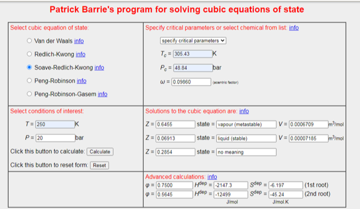
The Soave-Redlich-Kwong and the Peng-Robinson equation of states can accurately describe both the liquid and vapor phase. Here, we apply these two equations of state to estimate the molar volume of ethane. The liquid and gas molar volumes (in /mol) of ethane at the selected temperature (in K) and pressure (in bar) are obtained using the command NSolve as well as the Homotopy method described in detail in Ref. 1. Results are checked against their counterparts obtained using various online calculators.
3
cm
SRK EoS
SRK EoS
Tc=273.15+32.28;Pc=48.84;ω=0.09860;(*Ethane'scriticaltemperatureandpressureandacentricfactor*)R=83.14;(*universalgasconstantinbar*cm3/K*mol*)Tre=T/Tc;(*reducedtemperature*)Pre=P/Pc;(*reducedpressure*)
Parameters of the SRK Eos
b=0.08664RTc/Pc;m=0.480+1.574ω-0.176ω^2;a=0.42748(RTc)^2/Pc1+m1-
Tre
^2;In[]:=
Tc
Out[]=
305.43
In[]:=
T=250.;
In[]:=
Tre
Out[]=
0.818518
In[]:=
P=20;
In[]:=
Pre
Out[]=
0.4095
In[]:=
NSolve[P==RT/(v-b)-a/(v(v+b)),v](*molarvolumesusingNSolve*)
Out[]=
{{v670.848},{v296.559},{v71.8438}}
In[]:=
g[v_]:=Pv-RT(*idealgaslaw*)
In[]:=
f[v_]:=Pv-RTv/(v-b)+a/(v+b)
In[]:=
h[v_,t_]:=tf[v]+(1-t)g[v](*Homotopyfunction*)
In[]:=
MyGrad[fon_,var_List]:=D[fon,#]&/@var(*Jacobianmatrix*)
In[]:=
J=MyGrad[h[v,t],{v,t}]
Out[]=
20(1-t)+t20-+-,20785.-+
20785.
-45.0469+v
20785.v
2
(-45.0469+v)
6.34584×
6
10
2
(45.0469+v)
20785.v
-45.0469+v
6.34584×
6
10
45.0469+v
s is a continuation parameter
In[]:=
Js=J/.vv[s]/.tt[s]
Out[]=
20(1-t[s])+t[s]20-+-,20785.-+
20785.
-45.0469+v[s]
20785.v[s]
2
(-45.0469+v[s])
6.34584×
6
10
2
(45.0469+v[s])
20785.v[s]
-45.0469+v[s]
6.34584×
6
10
45.0469+v[s]
In[]:=
Eq[1]=D[v[s],{s,1}]First[Drop[Js,1]]
Out[]=
′
v
20785.v[s]
-45.0469+v[s]
6.34584×
6
10
45.0469+v[s]
In[]:=
Eq[2]=D[t[s],{s,1}]-First[Drop[Js,{2}]]
Out[]=
′
t
20785.
-45.0469+v[s]
20785.v[s]
2
(-45.0469+v[s])
6.34584×
6
10
2
(45.0469+v[s])
WhenEvent keeps track of the molar volumes obtained for t=1
In[]:=
{sol,points}=Flatten[Reap@Quiet@NDSolve[{Eq[1],Eq[2],t[0]0,v[0]RT/P,WhenEvent[t[s]==1,{Sow[{t[s],Log[v[s]]}]}]},{v,t},{s,-0.20,0.10}],1]
Out[]=
vInterpolatingFunction,tInterpolatingFunction,{{1.,6.50854},{1.,5.69225},{1.,4.27449}}


In[]:=
data=Table[Evaluate@{t[s],v[s]}/.sol,{s,-0.115,0.075,0.00001}];
All three molar volumes
In[]:=
points
Out[]=
{{1.,6.50854},{1.,5.69225},{1.,4.27449}}
As expected we find three roots when t=1; log scale is used for clarity
In[]:=
plt2=Show[ListLogPlot[data,AspectRatio->1,AspectRatio->1,Frame->True,GridLines->Automatic,PlotStyle->Darker@Red,Joined->True],PlotRange->{{-3,4},Automatic},Epilog->{PointSize[0.025],Darker@Green,Point[points[[1]]],Point[points[[2]]],Point[points[[3]]],Dashed,Darker@Blue,Line[{{1,-20},{1,20}}]},FrameLabel->{Style["t",16,Italic],Style["molar volume",16]},ImageSize->450{1,1},PlotLabel->Row[{Style["molar volumes in cm3/mol :",14,Darker@Red]," ",Style[E^points[[1,2]],Darker@Magenta,14]," ",Style[E^points[[2,2]],Darker@Green,14]," ",Style[E^points[[3,2]],Darker@Blue,14]}]]
Out[]=
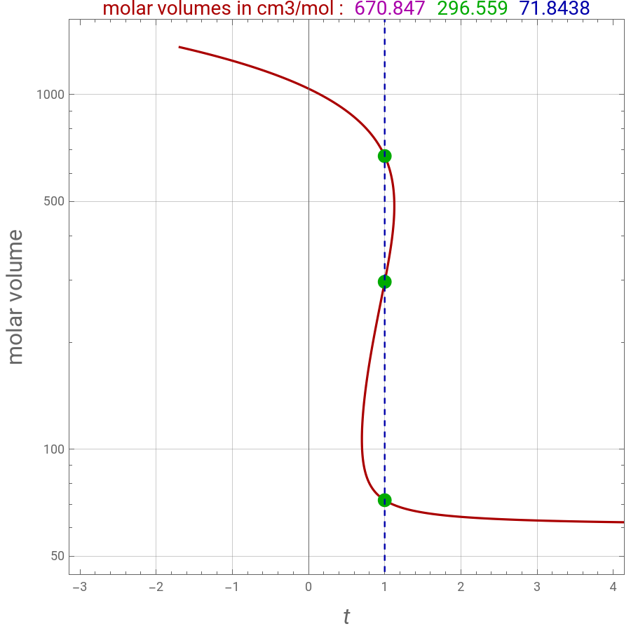
In[]:=
P{E^points[[1,2]],E^points[[2,2]],E^points[[3,2]]}/R/T(*compressibilityfactors*)
Out[]=
{0.645511,0.285359,0.0691304}
PR EoS
PR EoS
Parameters of the SRK Eos
b=0.07780RTc/Pc;m=0.37464+1.54226ω-0.26992ω^2;a=0.45724(RTc)^2/Pc1+m1-
Tre
^2;In[]:=
NSolve[P==RT/(v-b)-a/(v+(1+Sqrt[2])b)1/(v+(1-Sqrt[2])b),v](*molarvolumesusingNSolve*)
Out[]=
{{v652.874},{v282.536},{v63.3901}}
In[]:=
g[v_]:=Pv-RT(*idealgaslaw*)
In[]:=
f[v_]:=Pv-RTv/(v-b)+av/(v+(1+Sqrt[2])b)1/(v+(1-Sqrt[2])b)
In[]:=
h[v_,t_]:=tf[v]+(1-t)g[v](*Homotopyfunction*)
In[]:=
MyGrad[fon_,var_List]:=D[fon,#]&/@var(*Jacobianmatrix*)
In[]:=
J=MyGrad[h[v,t],{v,t}]
Out[]=
20(1-t)+t20-+-+-(97.6565+v),20785.-+
20785.
-40.4507+v
20785.v
2
(-40.4507+v)
6.65482×v
6
10
(-16.7552+v)
2
(97.6565+v)
6.65482×
6
10
(-16.7552+v)(97.6565+v)
6.65482×v
6
10
2
(-16.7552+v)
20785.v
-40.4507+v
6.65482×v
6
10
(-16.7552+v)(97.6565+v)
s is a continuation parameter
In[]:=
Js=J/.vv[s]/.tt[s]
Out[]=
20(1-t[s])+t[s]20-+-+-(97.6565+v[s]),20785.-+
20785.
-40.4507+v[s]
20785.v[s]
2
(-40.4507+v[s])
6.65482×v[s]
6
10
(-16.7552+v[s])
2
(97.6565+v[s])
6.65482×
6
10
(-16.7552+v[s])(97.6565+v[s])
6.65482×v[s]
6
10
2
(-16.7552+v[s])
20785.v[s]
-40.4507+v[s]
6.65482×v[s]
6
10
(-16.7552+v[s])(97.6565+v[s])
WhenEvent keeps track of the molar volumes obtained for t=1
All three molar volumes
As expected we find three roots when t=1; log scale is used for clarity
CITE THIS NOTEBOOK
CITE THIS NOTEBOOK
All molar volumes by homotopy for ethane at 250 K and 20 bar
by Housam Binous and Ahmed Bellagi
Wolfram Community, STAFF PICKS, June 29, 2025
https://community.wolfram.com/groups/-/m/t/3488429
by Housam Binous and Ahmed Bellagi
Wolfram Community, STAFF PICKS, June 29, 2025
https://community.wolfram.com/groups/-/m/t/3488429