In[]:=
ClearAll["Global'*"]Remove[x]df[x_[t_]]=4*D[x[t],{t,2}]+2*D[x[t],{t,1}]+4*D[x[t],{t,0}]ih[t_]=-9E^(-t/4)Sin[t(Sqrt[15]/4)]df1s=FullSimplify[DSolve[df[x[t]]==ih[t],x,t]];Evaluate[x[t]/.df1s]sln={{x->Function[{t},(C[2]*Cos[(Sqrt[15]*t)/4])/E^(t/4)+(C[1]*Sin[(Sqrt[15]*t)/4])/E^(t/4)+((3/10)*(Sqrt[15]*t*Cos[(Sqrt[15]*t)/4]))/E^(t/4)]}};Evaluate[x[t]/.sln]Simplify[df[x[t]]/.sln]Simplify[df[x[t]]/.df1s]WolframAlpha["DSolve[4* D[x[t],{t,2 }] + 2* D[x[t],{t,1 }] + 4* D[x[t],{t,0 }]== -9 E^(-t/4) Sin[t(Sqrt[15]/4)],x,t]"]
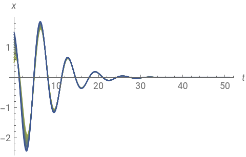
Out[]=
4x[t]+2[t]+4[t]
′
x
′′
x
Out[]=
-9Sin
-t/4
15
t4
Out[]=
Cos+Sin++2CosSin-2CosSin
-t/4
2
15
t4
-t/4
1
15
t4
3
10
-t/4
15
tCos15
t4
15
t2
15
t4
15
t4
15
t2
Out[]=
tCos+Cos+Sin
3
2
3
5
-t/4
15
t4
-t/4
2
15
t4
-t/4
1
15
t4
Out[]=
-9Sin
-t/4
15
t4
Out[]=
-9Sin
-t/4
15
t4
Out[]=