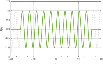
Force F(t) that last 10 cycles and angular frequency .
ω1
Ft=Sin[t]UnitBox;PlotSin[t],UnitBox,Ft,{t,-15π,15π},Frame->True,FrameLabel->{"t","F[t]"},PlotRange->{{-40,40},{-3/2,3/2}},Axes->False,GridLines->Automatic,PlotStyle->{{LightGray,Dashed},{LightGray,Dashed},}
t
20π
t
20π
Out[]=
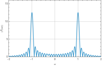
Compute the Fourier transform of the force:
Fω=FourierTransform[Ft,t,ω]
Out[]=
5
2π
Sinc[10π-10πω]-52π
Sinc[10π+10πω]Plot its absolute value:
AbsFω=Abs[Fω];Plot[AbsFω,{ω,-2,2},Frame->True,FrameLabel->{"ω","| (ω) |"},PlotRange->{{-2,2},{0,16}},Axes->False,GridLines->Automatic]
F
Out[]=
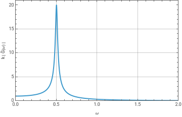
Now, say that applied this force to an underdamped harmonic oscillator of natural frequency 1/2 and a quality factor of approximately 20. (The precise value does not matter for our discussion). The expression for was derived in class.
ω
N
|(ω)|G(ω)
G
k=1;ωn=1/2;ζ=1/40;AbsGω=;Plot[AbskGω,{ω,0,2},Frame->True,FrameLabel->{"ω","k | (ω) |"},PlotRange->{{0,2},{0,21}},GridLines->Automatic]
1
k
1
Sqrt[+]
2
(1-)
2
(ω/ωn)
2
(2ζω/ωn)
G
Out[]=
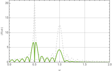
To find the (absolute value) of the Fourier domain representation of the position, (ω), we multiply the absolute values of the Fourier transformation of the force, (ω), and of the response function, (ω). In the plot below, we plot the latter two in dashed gray curves, they product is the green curve.
x
F
G
Plot[{AbskGω,AbsFω,AbskGω*AbsFω},{ω,0,2},Frame->True,FrameLabel->{"ω","| (ω) |"},PlotRange->{{0,2},{0,21}},GridLines->Automatic,PlotStyle->{{LightGray,Dashed},{LightGray,Dashed},}]
x
Out[]=