This book provides a concise and practical introduction to quantum computing, emphasizing an interactive, hands-on approach. It introduces and explores the essential concepts, principles, and foundational quantum algorithms through guided modeling and simulation exercises. Each topic is developed computationally, allowing readers to build both intuition and technical proficiency by directly engaging with the computational mechanics of quantum systems. The approach taken here is computation first, meaning that understanding arises through the act of calculation, echoing David Mermin’s well-known slogan, “shut up and calculate.”
Full book: https://wolfr.am/QC-Book
Community post of part 2: https://community.wolfram.com/groups/-/m/t/3587994
Community post of part 2: https://community.wolfram.com/groups/-/m/t/3587994
Who is this book for? It is written for anyone curious about learning quantum computation through the lens of discrete vector spaces, seasoned with a delightful touch of quantum computing. I have deliberately avoided delving into the nitty-gritty of mathematical formalism. Instead, my focus is on computation itself, on doing the work, even when the underlying mathematics is complex and hidden behind the scenes. As I mentioned in the abstract, I believe one of the most important steps in learning quantum theory (an abstract and often intimidating subject at first encounter) is to learn by doing the computations.
The environment you will be working in is a Mathematica notebook. Every Mathematica notebook is organized into cells, each marked by a small bracket along the right edge of the window. A cell can contain text, visualizations, data, input code, or nearly anything else that can be expressed in computational form. In essence, it is a flexible workspace where ideas, mathematics, and computation come together seamlessly.
Many of the calculations in this book will be carried out using the Wolfram Quantum Framework. This framework is distributed as a paclet, meaning it is a collection of specialized functions. Once installed, these functions and their documentation pages become integrated into Mathematica, just like its native built-in functions. Do not get intimated by code. Even if it looks complicated, for many parts you can ignore the code and focus on the outcome.
If any question, please reach out to quantum@wolfram.com
Table of Contents (Part 1)
What Is Quantum Computation?
We begin with a brief revisit of classical computation through a series of hands-on examples. From there, the focus transitions to the quantum domain, where you will explore several examples of quantum circuits. Each example is accompanied by corresponding code; it’s perfectly fine if not everything is immediately clear. As you move forward, your grasp of quantum principles and your coding proficiency will develop together, reinforcing one another through practice and exploration.
Key Concepts
Key Concepts
◼
Classical computation
◼
Quantum computation
◼
Quantum bit (qubit)
◼
Quantum circuit
Classical Computation
Classical Computation
In order to understand quantum computation, it helps to compare it to classical computation. To compute something, you have to be able to use rules to determine what should be the output from a list of inputs. You can think of computing as starting with the inputs and following the rules to reach an output.
Consider two binary numbers “01” and “10” and let’s see how we can add them. First, each bit-string is interpreted as a base-2 number rather than ordinary decimal, so “01” becomes one and “10” becomes two.
Define binary strings:
In[]:=
a="01";b="10";
Construct the number from the base-2 digits of :
a
In[]:=
FromDigits[a,2]
Out[]=
1
Construct the number from the base-2 digits of :
b
In[]:=
FromDigits[b,2]
Out[]=
2
Add the numbers using normal addition:
In[]:=
FromDigits[a,2]+FromDigits[b,2]
Out[]=
3
Convert the total back into bit-string:
In[]:=
IntegerString[FromDigits[a,2]+FromDigits[b,2],2]
Out[]=
11
To get a better sense of constructs of numbers in a base , let’s consider symbolic digits and base:
b
In[]:=
ExpandFromDigitsc.4,c.3,c.2,c.1,c.0,b.
Out[]=
c.0+b.c.1+c.2+c.3+c.4
2
b.
3
b.
4
b.
Donating the length of digits by , the maximum power of will be (in the above example, ).
n
b
n-1
b
5-1
b
Let’s consider another example. Add two binary strings 100 and 011:
In[]:=
a="101";b="011";IntegerString[FromDigits[a,2]+FromDigits[b,2],2]
Out[]=
1000
Note that something interesting happened in above calculation. Pay attention to the string length of initial numbers and final total. The original bit-strings had the string length of 3 while the final answer is a four-bit string. Let’s dive in a bit more.
What are all the states of a sequence of three classical bits?
In[]:=
threeBits=Tuples[{0,1},3]
Out[]=
{{0,0,0},{0,0,1},{0,1,0},{0,1,1},{1,0,0},{1,0,1},{1,1,0},{1,1,1}}
What are the corresponding numbers from above base-2 digits?
In[]:=
FromDigits[#,2]&/@threeBits
Out[]=
{0,1,2,3,4,5,6,7}
With a 3-bit string you can represent 0–7; in general, n bits represent 0 to -1. Returning to the example, adding 101 and 011 gives 8, which exceeds the 3-bit range. This means in-place addition is modulo , so the sum wraps to 000 unless you provide an extra bit to capture the carry.
n
2
n
2
In[]:=
FromDigits[a,2]+FromDigits[b,2]
Out[]=
8
To encode that result as a bitstring, we need at least 4 bits (since 8 requires 4-bit representation).
In[]:=
IntegerString[FromDigits[a,2]+FromDigits[b,2],2]
Out[]=
1000
If you insist on staying within 3 bits, perform all operations modulo 8 (wrap-around arithmetic).
In[]:=
ModFromDigits[a,2]+FromDigits[b,2],
3
2
Out[]=
0
Then the 3-bit string of the above result is:
In[]:=
IntegerString[0,2,3]
Out[]=
000
Now let’s try another encoding scheme.
It is also possible to encode information in such sequences of classical bits to represent problems of interest. For example, each of those bit sequences could also encode letter characters with a different encoding scheme:
In[]:=
AssociationMap[FromLetterNumber[FromDigits[#,2]]&,threeBits]
Out[]=
{0,0,0} ,{0,0,1}a,{0,1,0}b,{0,1,1}c,{1,0,0}d,{1,0,1}e,{1,1,0}f,{1,1,1}g
With yet another encoding scheme, those same bit sequences could represent colors with opacity:
In[]:=
AssociationMap[Apply[RGBColor,#]&,threeBits]
Out[]=
{0,0,0},{0,0,1},{0,1,0},{0,1,1},{1,0,0},{1,0,1},{1,1,0},{1,1,1}

Having seen how a 3-bit register cleanly enumerates eight distinct states and how different encodings map those states to numbers, letters, or colors, we now move to the quantum setting. There the same eight basis strings exist, but a 3-qubit register can also occupy complex superpositions of them, and even entangled combinations that have no classical analogue. The rules for storing and extracting information therefore change: measurement reveals a single basis outcome, while computation exploits interference among amplitudes.
Quantum Circuits and Qubits
Quantum Circuits and Qubits
Now we’ll dive directly into quantum computation. We’ll introduce common terms and concepts widely used in quantum information. Some details will be only briefly mentioned in this chapter. For each topic, we’ll highlight what to focus on for a first exposure, and later we’ll return to expand on each concept in more depth.
In quantum computing, information is encoded in quantum states, which we transform into new states through some operations (i.e., quantum gates) tailored to a computational goal. Both states and transformations (i.e. their gates) have useful visual representations. In this chapter, we will emphasize visual intuition first and introduce the detailed mathematics later.
Since we will use the Wolfram Quantum Framework, we first need to install it.
In[]:=
PacletInstall["https://www.wolfr.am/DevWQCF",ForceVersionInstall->True]<<Wolfram`QuantumFramework`
Out[]=
PacletObject

The diagram below represents an example of a quantum circuit:
Out[]=
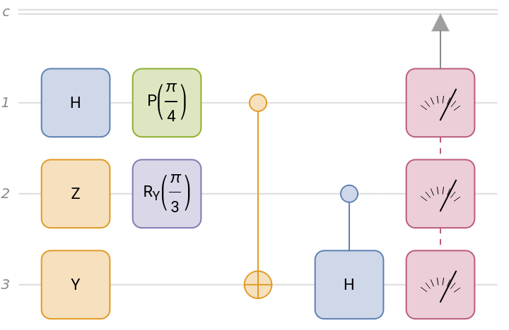
A quantum circuit is read from left to right. Looking into a quantum circuit, pay attention to wires, boxes, and how they are connected. The first operation, represented by the blue box labeled H, acts only on the first wire, while some operations act on more than one wire; they are multi-qubit gates. The boxes that look like gauges on the right hand side of the diagram represent measurement and point to the wire labeled . The wire labeled represents a classical system (such as part of a regular computer) where the results of the measurements on qubits are stored. All operations shown except for measurements are unitary and reversible, a key feature we’ll explore in more detail later. You can think of each box as performing a transformation on the quantum state of one or more wires. These transformations must obey fundamental principles dictated by quantum theory.
c
c
Notice how the circuit diagram has several wires, labeled , 1, 2 and 3. Wires 1, 2 and 3 represent qubits (quantum bits) instead of classical bits. They carry quantum data. The above circuit is a 3-qubit system, meaning that the state can be described in the complex vector space . There are 8 possible bitstrings for 3 classical bits.
c
8
In[]:=
StringJoin/@Tuples[{"0","1"},3]
Out[]=
{000,001,010,011,100,101,110,111}
These eight classical bits can form a convenient basis (usually called as the computational basis) for the complex vector space . Although the notation looks very similar to the classical one, but those 3-bits in quantum are represented by wrapping them around a notation which is called a ket. In general, a ket is a shorthand representation of a complex-valued vector, although a ket with n-bitstring represents a -dimensional unit vector. A general 3-qubit state is a complex linear combination of those eight basis states.
8
|…〉
n
Show the vectors corresponding to computational basis of 3-qubits:
Out[]=
,
,
,
,
,
,
,
000
1 |
0 |
0 |
0 |
0 |
0 |
0 |
0 |
001
0 |
1 |
0 |
0 |
0 |
0 |
0 |
0 |
010
0 |
0 |
1 |
0 |
0 |
0 |
0 |
0 |
011
0 |
0 |
0 |
1 |
0 |
0 |
0 |
0 |
100
0 |
0 |
0 |
0 |
1 |
0 |
0 |
0 |
101
0 |
0 |
0 |
0 |
0 |
1 |
0 |
0 |
110
0 |
0 |
0 |
0 |
0 |
0 |
1 |
0 |
111
0 |
0 |
0 |
0 |
0 |
0 |
0 |
1 |
The quantum state of the above circuit, just before measurement, is:
Out[]//TraditionalForm=
1
2
3
2
4
4
1
2
3
2
π
4
1
4
π
4
1
4
π
4
The above representation illustrates quantum superposition, which is a linear combination of multiple states with coefficients that, in general, can be complex numbers.
What are the results of running this circuit? Since measurements are included at the end, executing the circuit returns a quantum measurement object in the Wolfram Quantum Framework. This object contains the probability distribution over possible bitstrings and can be sampled to generate measurement outcomes:
In[]:=
measurements=qc[]
Out[]=
QuantumMeasurement

Note that by executing the code above, we simulated a quantum computation on a classical computer. This is exactly what a quantum simulator does: it numerically emulates quantum state evolution and measurement according to the rules of quantum mechanics, all while running on classical hardware.
Alarm: saying we “performed a quantum computation” can be misleading, simulators do not provide quantum speedups, are limited by exponential memory growth with qubit count, and only capture noise or device effects if those are explicitly modeled.
What are the results of the measurement in this circuit?
Notice that the possible outcomes of a quantum measurement are simply classical bit sequences. In the earlier classical computation examples, the rules were deterministic: each input led to a definite output. In contrast, quantum computation typically yields a range of possible outcomes, each with a certain probability. This is because quantum theory provides a probabilistic description of measurement results, with the distribution determined by the state just before measurement (and the chosen measurement basis).
Additionally, you can compute how the quantum state evolves as gates are applied. Although we have not yet discussed the state in full detail, for now focus on the linear combination of computational-basis bitstrings and examine the coefficient (amplitude) of each term. These amplitudes update linearly under gates, and their squared magnitudes determine the probabilities of the corresponding bitstrings upon measurement.
Keep in mind that, in the end, the most important information we extract from a quantum system is its measurement results (and their statistics). We will discuss this in more detail in future chapters.
Quantum States: Single Particle Case
We review quantum states for a single system: state vectors, amplitudes, and measurement probabilities. We then contrast pure and mixed states and describe both with the density matrix. Finally, we extend these ideas to higher-dimensional systems.
Key Concepts
Key Concepts
◼
Quantum State
◼
Amplitudes
◼
State Vector
◼
Dirac Notation
◼
Bloch Sphere
◼
Density Matrix
◼
Pure vs Mixed States
Bloch Sphere
Bloch Sphere
Qubits are not classical bits, so listing classical bitstrings does not capture all possible qubit states. How are quantum states represented instead? Let’s begin with some visual intuition. There is a very useful graphical representation of 1-qubit states called the Bloch sphere. The Bloch sphere is named after physicist Felix Bloch:
In this approach, a quantum state is represented by a point in 3D space inside a sphere of radius 1 (the Bloch sphere). The point may lie on the surface, in which case we call it a pure state, or inside the sphere, in which case we call it a mixed state.
Bra-Ket Notation
Bra-Ket Notation
Another common notation in quantum is the bra–ket notation. It is also called the Dirac, after the famous British physicist, Paul M. Dirac.
Show the matrix form and also Dirac notation of NOT gate:
Show the Dirac notation of controlled-Hadamard gate:
Show the matrix of controlled-Hadamard gate in the computational basis:
State Vectors, Amplitudes and Density Matrices
State Vectors, Amplitudes and Density Matrices
Now consider the result of applying a Hadamard gate to the register state of a qubit:
If the initial state isn’t specified, Wolfram’s Quantum framework initializes the n-qubit register to the all-zeros state.
The coefficients of each basis element are known as the quantum amplitudes. A quantum state can be defined by giving its amplitudes:
The above state can be written in Dirac notation:
Notice the relationship between the vector coefficients and the probabilities according to the Born’s rule:
Probabilities are also basis-dependent; unless specified otherwise, they are computed in the computational basis. For example, transform the same state into Pauli-Y basis and calculate the probabilities:
We will discuss the basis transformation later.
Calculate probabilities in the computational basis for a quantum state:
Calculate probabilities in the computational basis for another quantum state:
Although the state vectors above are different, their computational-basis outcome probabilities are identical. This highlights a key point: measurement probabilities are basis-dependent. Next, compute the probabilities of these two states in the Pauli-X basis.
This is a subtle but important point: measurement probabilities are basis-dependent. In the Pauli-X basis, the distinction between the two states is clear, because their outcome probabilities differ.
Given a state vector, one can calculate probabilities manually too:
For probability calculations, always use a normalized state (or normalize the probabilities at the end).
However, there are situations where describing a qubit by a 2-vector is not enough. For example, in the famous Stern–Gerlach experiment—where a beam of silver atoms is sent through an inhomogeneous magnetic gradient—the initial state of the atoms, even if approximated by their electron spin only, may be an ensemble rather than a single pure state.
In such cases, a state vector cannot fully describe the system. Instead, we use a density matrix (or density operator). The demonstration above is modified from an example in the Wolfram Demonstration Project.
Generate a state using above state vector:
Compute the measurement probabilities in the computational basis:
Using this result, now compute the measurement probabilities in the Pauli-X basis:
The result shows that this pure state cannot yield 1/2 measurement probabilities in every basis. This motivates the more general description of quantum states using a density matrix. For example, let’s define a state by half of identify matrix:
Notice the tag “Mixed state” in the summary box of quantum state above.
The Dirac notation of the state is simply the density matrix written in the computational basis.
Now we can show that the measurement probabilities are the same in every basis and equal to 1/2.
An interesting feature of mixed states is that they lie inside the Bloch sphere, whereas pure states (those describable by a single 2-vector) lie only on the surface.
Show the Bloch vector of a mixed state:
Calculate purity for a pure state:
In summary, when thinking about the state of a qubit, you can view it in several equivalent ways:
◼
As a linear combination (a complex-valued 2-vector) in a given basis.
◼
As a real-valued 3-vector representing Cartesian coordinates of the Bloch vector {x,y,z}.
◼
As the same point in spherical coordinates {r,ϕ,θ}.
Generate different representations of a random state:
Pauli operators and Bloch sphere
Pauli operators and Bloch sphere
Pauli operators provide a natural choice for representation of the density matrix:
Check that Pauli matrices are Hermitian:
Find the eigensystem of Pauli-Z:
Verify the −1 eigenvalue by applying the operator to the candidate state and confirming the result is exactly the original state multiplied by −1 (same amplitudes, same relative phases, overall sign flip only):
Verify the +1 eigenvalue by applying the operator to the candidate state and confirming the output equals the input (no change in amplitudes or relative phases).
From now on, unless stated otherwise, we will choose eigenvectors to be normalized. The eigenvectors then form an orthonormal basis for the vector space.
We will call the eigenvector with the positive eigenvalue as by + subscript and the negative one by - subscript. Putting this together, we can represent the Bloch-sphere positions of the eigenvectors of the Pauli operators as follows:
Each of the six states shown above lie along the Cartesian axes of the sphere. For various historical reasons, these states have alternate names in the context of quantum computing.
Note that Pauli-Z eigenvectors are the same as the computational basis:
Higher Dimensions
Higher Dimensions
The simplest quantum system is a qubit, represented by a two-dimensional complex vector space. For example, show the T-type magic state’s amplitudes in the computational basis:
Quantum systems can also be higher-dimensional; a three-level system is called a qutrit, such as a spin-1 system.
Applying the qutrit (3D) Hadamard to the 0 state yields an equal superposition of all three basis states, each with the same magnitude and evenly spaced relative phases:
For the 3D Hadamard we use the same “H” symbol; the difference is that it acts on qutrit (3-level) wires rather than qubit wires.
Pay attention to the notation for the corresponding basis:
Show the matrix form of the 3D Hadamard:
Let’s focus on a special qutrit. A three-level lambda system (Λ system) is an atom or qutrit. Think of the levels forming the shape of the Greek letter Λ: the two lower “arms” meet at the upper “node.” Two lasers are used, one drives the left lower state to the excited state (pump), the other drives the right lower state to the excited state (Stokes).
This setup is a workhorse in quantum optics because it lets you move population or create superpositions between the two stable lower states while keeping the fragile excited state mostly unoccupied, enabling techniques like Stimulated Raman Adiabatic Passage (STIRAP), electromagnetically induced transparency, and coherent population trapping.
Consider an operator as follows:
Find the eigensystem of the Hamiltonian:
As one can see, one of the eigenvectors correspond to the eigenvalue zero.
The above state is called a dark state. A dark state is a special superposition of the two long-lived ground states in a three-level Λ system that does not couple to the excited state under the applied lasers. Practically, the pump tries to lift amplitude from one ground state and the Stokes from the other; in the right superposition their effects on the excited level cancel by destructive interference, so the system does not absorb light.
Check the quantum states are the same:
Probability and Measurement
We will discuss the concept of probability and how it relates to the frequency of different outcomes in a repeatable measurement. Then we will show how probabilities in quantum theory help us calculate joint and marginal probabilities.
Key Concepts
Key Concepts
◼
Random Outcome, Probability Distribution, Marginal Probability, Joint Probability
◼
Marginal Probability
◼
Joint Probability
Frequency vs probability
Frequency vs probability
You’re no doubt familiar with coin flips or dice rolls as ways to generate random outcomes. For our purposes, think of a random outcome as a definite result from a repeatable experiment. Randomness here means that several different outcomes are possible, and while we may know their probabilities, there is no way to determine which specific outcome will occur before running the experiment.
You can find much more information on probability and statistics in any of the following Wolfram U courses: Introduction to Probability, and Introduction to Statistics.
Quantum theory provides a way to compute the probability distribution over possible measurement outcomes. You can think of a probability distribution as a rule that assigns a nonnegative probability to each possible outcome of an experiment, with all probabilities adding up to 1. In quantum circuits, this distribution is typically defined over the discrete set of possible bitstrings.
Let’s look at a couple examples of generating random outcomes to build intuition.
Suppose you want to sample a random integer between 1 and 10. One realization of this process is as follows:
The above function returns a uniformly random integer from 1 to 10 (inclusive).
Now examine the count of each number in the sequence above.
Now examine the frequency of each number in the sequence above:
Now examine the frequency of each number across different sequences as the sequence length increases:
As you can see, with more repetition of the same experiment, the observed frequency of outcomes gets closer to the true probability distribution.
Now let’s consider the case where we assign a specific weight to each number: {1,1,2,3,4,4,3,2,1,1}.
We can compute the corresponding probabilities by normalizing the weights; that is:
We can compute the corresponding probabilities by normalizing the weights; that is:
If we run the experiment many times, we expect the frequency of results to converge to the probabilities above. Now let’s generate different data samples of results for 10, 100, and 10,000 runs. As the number of realizations increases, the observed frequencies should get closer to the expected probabilities.
Calculate frequencies for each experiment:
Visualize the results:
As expected, with more runs of the experiment, the observed frequencies get closer to the expected probabilities (law of large numbers).
Now let’s consider a case analogous to three different players rolling dice and collecting their joint outcomes. Of course, the quantum case can differ markedly from the classical one—classically, similar correlations might require prearranged strategies or communication. For the moment, however, we will set aside interpretation and focus only on the probabilities of the outcomes (i.e., the joint distribution and any marginals), leaving the discussion of correlations for later.
Joint vs Marginal Probabilities
Joint vs Marginal Probabilities
We will prepare the system in a special initial state. For now, we will skip the details of what this state is and focus only on the probability of outcomes. Using quantum theory, we can calculate the joint probabilities of the measurement results, that is, the probabilities for all possible tuples of 0s and 1s listed above.
Generate the corresponding multivariate distribution of outcomes:
Visualize the contingency table of the distribution:
Since we have the multivariate distribution, we can compute the probability of any scenario by summing over the appropriate outcomes. Let’s consider a few cases.
Calculate the probability of getting 0 for qubit-1 and 1 for qubit-3 (and any result for qubit-2)
Let’s calculate the above probability step-by-step:
2
.Extract the probabilities associated with those selected outcomes.
3
.Add those probabilities together.
We can use the multivariate distribution and compute the full list of outcome–probability pairs:
Now suppose we do not care about qubit 3 and want to focus only on the statistics of qubits 1 and 2. To do this, we compute the marginal distribution by summing over the outcomes of qubit 3. (In the quantum formalism, this corresponds to taking the partial trace over qubit 3 to obtain the reduced state of qubits 1 and 2.)
To get the marginal distribution, the calculation as follows:
- first group outcomes based on the values of the first and second elements (we are only interested in the marginal distribution qubit 1 and 2)
- for each group, add up the values of probabilities
- first group outcomes based on the values of the first and second elements (we are only interested in the marginal distribution qubit 1 and 2)
- for each group, add up the values of probabilities
The same process can be done more cleanly using built-in Wolfram Language functionality. This makes it much easier to compute other probabilities as well (you’ll see this shortly).
Calculate the marginal distribution
Visualize the contingency table of the marginal distribution:
Calculate the probability of getting 0 for qubit-1 from the marginal probability distribution:
Calculate the probability of getting 0 for qubit-1 from the overall probability distribution:
Let’s focus again on the computation that we did for finding two-dimensional marginal distribution from the three dimensional one, by averaging over third system:
The analysis above used standard probability theory throughout; only the initial probabilities were derived from quantum mechanics. That said, the rules of quantum theory provide a recipe for obtaining the quantum state of qubits 1 and 2 by averaging over all contributions from qubit 3, and thus getting probabilities directly from a new quantum state. For this aim, one should trace over the degrees of freedom of qubit 3, which yields the reduced state for qubits 1 and 2.
Trace out the qubit-3 (which is the 3rd subsystem) from the overall state:
Note what happened: the three-qubit state was pure, but the reduced state of qubits 1 and 2 is mixed (after tracing out qubit 3, due to entanglement).
As expected, this reduced state yields the same marginal probabilities as before:
Show the probabilities obtained from marginal distribution:
In future chapters, we will discuss in details the idea of tracing out a subsystem and how to describe the state of composite systems in quantum theory.
Quantum States: Multi-Particle Cases
We will discuss the tensoring of vector spaces, which provides a recipe for constructing larger systems from smaller ones. This recipe comes with some unique features. For example, there exist states that cannot be written as a tensor product of smaller states. We will examine these states and their distinctive feature: entanglement.
Key Concepts
Key Concepts
◼
Tensor product
◼
Kronecker product
◼
Composite systems
◼
Separable states vs entangled states
Tensor Product Structure
Tensor Product Structure
Consider a quantum system that is a qubit. This means its state lives in a 2-dimensional Hilbert space. The corresponding computational basis elements are
Of course, quantum systems can have other dimensions. For example, consider a 3-dimensional Hilbert space (a qutrit). The corresponding computational basis elements are
Now consider a composite system made of two qubits. How can we construct the larger space from the Hilbert spaces of the single qubits? This is the fundamental idea behind the tensor product.
The exact computation for basis tensoring is done as follows:
There are some minor details regarding the shapes of arrays after tensoring, which we’ll skip for now. The good news is that this tensor-product structure is fully supported in the Wolfram Quantum Framework: you can obtain the corresponding computational basis of a composite system simply by supplying the dimensions of the subsystems. For example:
This idea of tensoring applies directly to quantum states and operators. For example, we can create the composite state of a two-qubit system from its subsystem states:
Show the traditional form of above composite state:
As another example, let’s create a composite (i.e., multi-particle) operator as Pauli-Z acting on qubit 1 and Pauli-Y acting on qubit 2:
Show the matrix form explicitly:
Separable vs Nonseparable Objects
Separable vs Nonseparable Objects
An important point is this: the larger space built from smaller spaces can contain elements (states or operators) that cannot be written as a simple tensor product of two elements. For now, we will focus only on quantum states.
Consider a uniform superposition of a two qubit system:
The above state can be obtained by two Hadamard operators acting on 2-qubit register state:
Create uniform superposition of qubit 1 and 2:
Create the corresponding tensor product state:
Check the new state is the same as the previous one:
How, in general, can we check whether a state is separable? A systematic way to handle the general cases is the Schmidt decomposition. It says that any two-part pure state can be expressed as a sum of paired basis states for the two subsystems, each paired term weighted by a nonnegative number called a Schmidt coefficient. The state is separable exactly when there is only one nonzero Schmidt coefficient. In that situation, the state reduces to a single paired basis term (often called the Schmidt basis form), which means it is a simple product state rather than an entangled one.
In the Wolfram quantum framework, you only need to transform the state into its Schmidt basis and check Schmidt coefficients.
Show the composite state after the Schmidt decomposition:
Show amplitudes in the Schmidt basis:
Now let’s consider another example. We will use one of Bell states
Show its Dirac notation:
As we can see from the Schmidt decomposition, there is more than one nonzero Schmidt coefficient. This means the state is not separable; in other words, it is entangled.
Check the state is entangled:
An important question is how to quantify entanglement. We will cover standard measures and criteria in the next chapter.
Superposition and Entanglement
We will discuss the concepts of quantum superposition and entanglement in more detail. We will show how a linear combination of quantum states can look different from one basis to another, and how this relates to whether states are separable or entangled. We will then explain how to test whether a state is entangled and how to quantify the amount of entanglement.
Key Concepts
Key Concepts
◼
Superposition
◼
Entanglement
◼
Partial Trace
Superposition
Superposition
Superposition and entanglement are two fundamental characteristic traits of the quantum world. Superposition is a direct consequence of the linearity of quantum dynamics, while entanglement stems from the tensor-product structure of the underlying vector spaces together with the linearity.
Check the final state of the circuit is a uniform superposition:
Show the Dirac notation in the corresponding basis:
This representation can also be misleading, because it is a linear combination (i.e., a quantum superposition) in the computational basis. If you rewrite the same state in a different basis, it may take a very different form.
Transform the state in the Pauli-X basis:
Transform the state in the Pauli-Y basis:
Given the infinite choices of bases to represent a state, which basis is most convenient for a given task? Let’s discuss practical criteria for choosing a basis.
Let’s consider the effect of phase operator on 1-qubit computational basis vs Pauli-X basis:
For the X-rotation gate, the Pauli-X eigenbasis is the most natural basis to describe its effect.
A basis transformation can be done also for a composite state. For example, consider the state coming out of this circuit:
Execute the circuit and show the Dirac notation of the state:
If we transform this state to the Pauli-X basis, the form of the superposition changes. In particular, if the state is an eigenstate of X, it appears as a single basis vector in the X-basis (so the superposition “disappears”). Otherwise, it remains a superposition—just expressed in terms of the X-basis vectors.
In other words, the representation of the state in the computational basis shows a superposition, so it is not immediately clear whether the state is a tensor product of two single-qubit states. However, if we rewrite the same state in another basis (for example, the eigenstates of Pauli-X) and the factorization becomes explicit, then the state is separable (not entangled) and can indeed be written as a tensor product. Note that separability is a property of the state itself, not the basis; a different basis can simply make that property more evident.
If a state is separable, we say it is not entangled.
One way to confirm that a state is separable (for pure states) is to trace out a subsystem and check that the resulting reduced state is the same single-system state you specified in the product. Equivalently, both reduced states are pure, which indicates the overall state is a product (not entangled).
Additionally, for separable states, the reduced state is a pure state:
Let’s discuss entanglement in more detail.
Entanglement
Entanglement
Entanglement is when a composite quantum system has a well-defined overall state, but its parts cannot be assigned complete, independent states.
To create an entangled state, you will need a gate that is not separable. A famous gate that can be used is CNOT. Let’s see the effect of CNOT on the computational basis:
Calculate the final state of above circuit:
Show it in the Dirac notation:
Calculate the corresponding measurement probabilities:
Consider the state one gets after measuring above state. This is usually called post-measurement state. It will be a mixed state of 00 and 11, with the corresponding probabilities. It can be written as:
As you can see, the mixed state yields the same measurement probabilities as the original state.
In other words, one instance of measurement statistics alone does not make it obvious whether the state is entangled.
Test if above pure state is entangled or not:
Test if above the post-measurement state is entangled or not:
For multi-qubit systems, be sure to specify the partition of subsystems when you call QuantumEntangledQ, (always check the documentation pages).
Another way to test whether a state is entangled is as follows. First, compute the reduced states by performing partial traces. Then compare the tensor product of the reduced states with the original state. If they are the same, the state is not entangled; otherwise, it is entangled.
Generate the reduced state of qubit 1:
Generate the reduced state of qubit 2:
Compare the tensor product of the reduced states with the original state:
Since they are not the same, it means the original state was entangled state.
The above criterion works only for pure states. For mixed states, however, separability does not generally imply equality with the product of the marginals (many separable mixed states are mixtures of product states), so additional tests are needed.
Show that above approach does not work for an initial mixed state:
So although the result is False, but the initial state is not entangled.
Last but not least, given an entangled state, an interesting question is to quantify the entanglement. One common measure is called the generalized concurrence, which is a measure for the entanglement monotone. See the documentation page of QuantumEntanglementMonotone for more details.
Calculate the concurrence for the above state:
Calculate the concurrence for the Bell state:
As you can see, the Bell state is maximally entangled, it exhibits the strongest possible two-qubit entanglement (e.g., one bit of entanglement entropy, concurrence equal to 1).
Entanglement can extend beyond only two qubits. The GHZ circuit is shown below:
The outcome of above circuit is a state is usually called as GHZ state:
We also have GHZ as a named state in the Wolfram quantum framework:
Check GHZ state is an entangled state:
Calculate its concurrence:
A Quick Tour of Quantum Gates
This chapter offers a streamlined overview of quantum gates, focusing first on single-qubit operations that create superposition and control phase, then on multi-qubit gates that generate and manipulate entanglement. We survey core primitives and how they compose into universal sets, highlighting the role of controlled interactions such as CNOT, CZ, and SWAP. The goal is to give readers a compact, working intuition for how quantum gates shape computation, from isolated rotations to coordinated, entangling dynamics.
Key Concepts
Key Concepts
◼
Quantum logic operations
◼
Single-qubit quantum gates
◼
Multi-qubit quantum gates
Introduction
Introduction
Quantum circuits are usually represented using conventional names for the corresponding gates. For example, consider the circuit below:
Single-Qubit Gates
Single-Qubit Gates
Single-qubit gates are the building blocks of quantum computation. Each one acts on a single qubit, changing its state without touching the rest of the qubits. You can think of them as moving of a point on the Bloch sphere, steering a qubit from one configuration to another while preserving quantum amplitudes overall. Because any multi-qubit algorithm ultimately relies on carefully shaped single-qubit transformations combined with entangling operations, mastering these gates is essential for designing circuits, controlling interference and preparing useful superpositions.
In practice, single-qubit gates include familiar primitives like Pauli X, Y, and Z, which implement axis flips; the Hadamard, which creates and removes balanced superpositions; phase-type gates such as S and T that adjust relative phase without changing measurement probabilities; and continuously tunable rotations that let hardware enact arbitrary angles around chosen axes. Together they form a universal toolkit for shaping quantum states: calibrating amplitudes, sculpting phases, and setting up interference patterns that later multi-qubit gates can exploit.
Pauli gates
Pauli gates
Pauli operators are a common set of single-qubit gates. The Pauli-Z operator acts like a phase flip: it leaves the 0 state unchanged and adds a minus sign to the 1 state. In other words, if a qubit has some amount of 0 plus some amount of 1, applying Z keeps the 0 part the same and flips the sign of the 1 part. (By comparison, X swaps the 0 and 1 states, and Y also swaps them but introduces a phase.)
Effect of Pauli-Z on the state vector:
Effect of Pauli-Z in the Dirac notation:
The Pauli-Z gate is equivalent to a phase rotation by an angle of pi. Aside from an overall global factor (a “global phase” that doesn’t affect measurement outcomes), they act the same on any qubit: the 0 part is unchanged, and the 1 part picks up a minus sign.
Effect of Phase-π gate in the Dirac notation :
Additionally, Pauli-Z operator can be seen as flipping eigenstates of Pauli-X
The Pauli-Z gate turns the plus state (the equal mix of 0 and 1 with the same sign) into the minus state (the equal mix of 0 and 1 with opposite signs)
Check that applying the Pauli-Z gate to the plus state returns the minus state.
The Pauli-Z gate turns the minus state (equal mix of 0 and 1 with opposite signs) into the plus state (equal mix with the same sign).
Check that applying the Pauli-Z gate to the minus state returns the plus state.
Let’s visualize the effect of the Pauli-Z gate on different states by comparing the Bloch vectors of the initial and final states.
Pauli-X is also called the “NOT” operator because it acts like a NOT gate on the computational basis.
Check that applying Pauli-X to the 0 state yields the 1 state.
Check that applying Pauli - X to the 1 state yields the 0 state .
Let' s visualize the effect of the Pauli - X gate on different states by comparing the Bloch vectors of the initial and final states .
Pauli-Y on the 0 state acts like a phase-sensitive flip: it turns 0 into 1, up to an overall phase.
Similarly, Pauli-Y on the 1 state acts like a phase-sensitive flip: it turns 0 into 1, up to an overall phase.
Let' s visualize the effect of the Pauli - Y gate on different states by comparing the Bloch vectors of the initial and final states. Note that for the computational basis, the overall phase is not observable.
Hadamard gate
Hadamard gate
Another important single-qubit gate is the Hadamard gate.
This gate transforms a register state into a uniform superposition state.
Check the result is truly a uniform superposition:
Show the effect of H-gate on a generic quantum state:
Show matrix form of H-gate:
Family of phase-like gates
Family of phase-like gates
The phase gate is another important single-qubit gate.
It introduces a phase on the 1 state.
Show the matrix form of phase gate:
The S gate is another important single-qubit gate.
It introduces a phase on the 1 state.
Show matric form of S-gate:
S gate is the same as phase-π/2 gate:
The T gate is another common single-qubit gate.
It also introduce a phase on the 1 state.
Show matrix forma of T gate:
T gate is the same as phase - π/4 gate :
The label for the gate is obtained as follows:
Show that the phase shift is similar to a phase operator:
A special case of adding a phase is adding a global phase. This is what we usually call a global phase gate.
Since the phase is global (the same factor in front of all terms in the linear combination), it is not observable—it does not change the physical state.
Family of rotation gates
Family of rotation gates
Rotation around x-axis:
Show the effect of X-rotation on a generic quantum state:
Show the matrix form of x-rotation:
As mentioned before, an x-rotation is a rotation around the x-axis on the Bloch sphere.
Rotation around y-axis:
Show the effect of y-rotation on a generic quantum state:
Show the matrix form of y-rotation:
As mentioned before, an y-rotation is a rotation around the y-axis on the Bloch sphere.
Rotation around z-axis:
Show the effect of z-rotation on a generic quantum state:
Show the matrix form of x-rotation:
As mentioned before, an z-rotation is a rotation around the z-axis on the Bloch sphere.
The U3 gate is a general single-qubit rotation formed by combining the earlier rotations. It is defined by three angles.
Show the matrix forma of U3:
For example, generate three angles, and a point on the Bloch sphere:
Visualize the 3D point and its corresponding Bloch vector:
Visualize the transformed point using Euler rotations and the corresponding Bloch vector after U3:
A special case of the U3 gate is the U2 gate, specified by two angles.
Show matrix form of U2:
Multi-Qubit Gates
Multi-Qubit Gates
We now focus on multi-qubit gates. These are gates that cannot be written as a simple tensor product of single-qubit gates. Among multi-qubit gates, conditional (controlled) gates are especially important, because they serve as universal entanglers. Practically, you can take any of the single-qubit gates discussed before and make a controlled version. You designate a control qubit and a target qubit: the gate checks whether the control is in 0 or 1, and then, depending on the choice, control-0 (if the control is 0) or control-1 (if the control is 1), it applies the chosen gate to the target qubit.
Family of control NOT
Family of control NOT
CNOT (or CX) flips the target qubit when the control qubit is in the 1 state.
How CNOT transform 2-qubit computational basis:
CNOT is the same as CX:
Show the matrix form of CNOT gate:
As mentioned earlier, CNOT is one of the most important multi-qubit gates for generating entangled states. Example: prepare two qubits in a product state by putting qubit 1 into a uniform superposition with a Hadamard gate and leaving qubit 2 in the 0 state.
Check if this state is entangled or not:
Apply CNOT gate on the state and check if it is entangled or not:
As one can see, the CNOT gate transforms the state into an entangled state.
C0-NOT (or C0-X) flips the target qubit when the control qubit is in the 0 state.
How C0-NOT transforms 2-qubit computational basis:
Show the matrix form of C0-NOT gate:
Family of control phase
Family of control phase
Conditional Pauli-Z gate:
How CZ transforms 2-qubit computational basis:
Show the matrix form of CZ gate:
Conditional phase gate:
How CP transforms 2-qubit computational basis:
Show the matrix form of CP gate:
SWAP gate:
How SWAP transforms 2-qubit computational basis:
Show the matrix form of SWAP gate:
Root-SWAP gate:
How Root-SWAP transforms 2-qubit computational basis:
Show the matrix form of Root-SWAP gate:
Family of control rotation
Family of control rotation
Conditional rotation gate with Pauli-Z:
Ising-type entanglers are two-qubit unitaries generated by Pauli product interactions. They are like time evolutions under an “Ising” Hamiltonian. Any nontrivial angle produces entanglement; at special angles they’re locally equivalent to familiar gates such as CNOT. They are also native gates to many types of quantum hardware.
Family of Ising rotation
Family of Ising rotation
Ising ZZ (pure conditional phase):
Ising YY:
Ising XX:
3-qubit gates and more
3-qubit gates and more
Show Toffoli’s matrix form:
Show how a Toffoli gate acts on the computational basis of three-qubits:
Toffoli gate can be decomposed in terms of single-qubit gates and CNOTs as follows:
Show the above circuit acts the same as Toffoli:
Another important 3-qubit gate is Fredkin gate. It is also called CSWAP gate because it is conditional SWAP gate that conditionally exchanges two qubits. It is used in swap-test, data movement, and reversible sorting/comparison.
Show Fredkin’s matrix form:
Show how a Fredkin gate acts on the computational basis of three-qubits:
Fredkin gate can be also decomposed in terms of single-qubit gates and CNOTs as follows:
Show the above circuit acts the same as Fredkin:
CITE THIS NOTEBOOK
CITE THIS NOTEBOOK
Introduction to quantum computing: part 1
by Mads Bahrami
Wolfram Community, STAFF PICKS, December 9, 2025
https://community.wolfram.com/groups/-/m/t/3587974
by Mads Bahrami
Wolfram Community, STAFF PICKS, December 9, 2025
https://community.wolfram.com/groups/-/m/t/3587974