This project demonstrates how computational methods can be used to investigate protein structure beyond simply overall amino acid sequence analysis. We developed a series of custom Wolfram Language functions to automate protein retrieval, calculate amino acid abundance in percentage, extract α-helices, β-sheets, and loop regions, and visualize their compositions using percentage bar charts and ternary plots. Applying this code to a very well-known protein such as healthy and sickle-cell hemoglobin demonstrated that analyzing proteins at the secondary structure level provides greater insight than examining the complete sequence alone. The ternary plot revealed that the majority of amino acid changes remained concentrated within α-helical regions, while comparatively fewer changes occurred in loop regions and virtually no changes were observed within β-sheets. These findings are consistent with the known molecular mechanism of sickle-cell disease, where a single surface mutation promotes hemoglobin polymerization without substantially altering the protein’s overall secondary structure. Overall, this computational essay provides a framework for investigating the biological basis of proteins and can be readily extended to other proteins to explore relationships between sequence, structure, and disease.
Introduction
Introduction
Proteins are among the most essential biological macromolecules, and they carry out a range of functions necessary for human life. They can act as enzymes that catalyze biochemical reactions, provide structural support to cells and tissues, transport molecules throughout the body, and aid in signaling molecules that regulate cellular communication (Clinic, 2025). Every protein is composed of a unique sequence of amino acids, whose chemical properties determine how the protein folds into a specific three-dimensional structure. The sequence of amino acids in a protein is fundamental as even minor changes in the sequence can alter factors such as the protein’s stability, folding, and biological activity (Smith, 2017).
The structure of a protein is commonly denoted by four hierarchal levels, where the secondary structure represents localized folding patterns that are stabilized by hydrogen and peptide bonds. The three primary elements that make up the secondary structure of proteins include: α-helices, β-sheets, and loops. Certain amino acids preferentially occur within α-helices due to their ability to stabilize helical conformations, whereas other amino acids are more frequently found in β-sheets or flexible loop regions (Modeling, 1987). Analyzing the amino acid composition of individual secondary structures provides valuable insight into protein behavior.
One specific protein whose structure is particularly important to human health is hemoglobin, which is the oxygen transport protein found in red blood cells. Hemoglobin is responsible for transporting oxygen from the lungs to the tissues throughout the body and returning carbon dioxide to the lungs for exhalation. The normal adult form of the protein is predominantly composed of α-helices that aid in efficient oxygen binding and transport throughout the body. However, a single amino acid substitution mutation that occurs in the normal form specifically in the β-globin chain where glutamic acid is replaced by valine it produces the mutated form of hemoglobin (HbS). Although this mutation only affects one residue it alters the intermolecular interactions, promoting the aggregation of of hemoglobin molecules into rigid fibers under low-oxygen conditions. These fibers distort red blood cells into the characteristic sickle shape which gives rise to sickle cell disease, a hereditary disorder associated with chronic anemia, painful vaso-occlusive crises, and progressive organ damage (Mandal et al., 2020).
Understanding how amino acid composition relates to secondary structures in proteins is therefore an important step towards understanding the molecular basis of protein function and disease. Computational analysis provides an efficient means of investigating these relationships by extracting structural information directly from experimentally determined protein models and quantifying the distribution of amino acids within these structural regions.
Extracting Protein Data and Percent Composition Graphing
Extracting Protein Data and Percent Composition Graphing
Fetching Protein Entities
Fetching Protein Entities
Proteins are complex biological macromolecules, and their three-dimensional structures are stored globally in the Protein Data Bank (PDB). Every time a researcher uses techniques like x-ray crystallography or Cryo-EM to deduce the exact shape of a protein down to the individual atom, they upload that data to the PDB database and give it a unique 4-character alphanumeric identifier which is called a PDB ID (Berman, 2000). A standard entry in the PDB does not just contain a string of letters; rather, it maps out the exact X,Y, and Z spatial coordinates of every single atom in the protein. When these identifiers are called in the Wolfram language, the system connects directly to this global repository, allowing for the extraction of the primary amino acid sequences from the protein.
To explore the structural breakdown of sickle cell anemia, two distinct forms of human hemoglobin can be retrieved from the PDB database:
1. Normal Adult Hemoglobin (HbA) - This is represented by the PDB ID “1A3N”
2. Mutated Sickle Cell Hemoglobin (HbS) - This is represented by the PDB ID “2HBS”
1. Normal Adult Hemoglobin (HbA) - This is represented by the PDB ID “1A3N”
2. Mutated Sickle Cell Hemoglobin (HbS) - This is represented by the PDB ID “2HBS”
Import downloads the PDB file to isolate the multi-chain amino acid fragments, merging them into a single strand called healthySeq:
In[]:=
healthySeq=StringJoin[Import["https://files.rcsb.org/download/1A3N.pdb","Sequence"]];
StringTake cuts the 1148-letter mutated sequence down to the first 572 to isolate just one standard hemoglobin molecule:
In[]:=
mutatedSeq=StringTake[StringJoin[Import["https://files.rcsb.org/download/2HBS.pdb","Sequence"]],572];
StringLength counts the characters in both sequences to output a list containing the total number of amino acid residues for each:
In[]:=
{StringLength[healthySeq],StringLength[mutatedSeq]}
Out[]=
{572,572}
LetterCounts counts how many times each amino acid appears in the sequence and stores the totals in an association:
In[]:=
healthyAbundance=LetterCounts[healthySeq]
Out[]=
A72,L72,V60,K44,G40,H38,T32,S32,F30,D30,P28,E24,N20,R12,Y12,Q8,C6,M6,W6
In[]:=
mutatedAbundance=LetterCounts[mutatedSeq]
Out[]=
A72,L72,V64,K44,G40,H37,T32,S32,F30,D30,P28,E22,N20,R12,Y11,Q8,C6,M6,W6
The list of each of the corresponding amino acids for each peptide alphabet can be referenced in the table below.
Out[]//TableForm=
Peptide Alphabet | Amino Acid Name |
A | Alanine |
R | Arginine |
N | Asparagine |
D | Aspartic Acid |
C | Cysteine |
E | Glutamic Acid |
Q | Glutamine |
G | Glycine |
H | Histidine |
I | Isoleucine |
L | Leucine |
K | Lysine |
M | Methionine |
F | Phenylalanine |
P | Proline |
S | Serine |
T | Threonine |
W | Tryptophan |
Y | Tyrosine |
V | Valine |
Graphically Calculating and Visualizing Amino Acid Abundance
Graphically Calculating and Visualizing Amino Acid Abundance
To quantitatively compare the amino acid composition of healthy and mutated hemoglobin, the raw amino acid sequence must first be made into a format that can readily interpreted. While the language itself provides functions for counting the occurrence of each amino acid within a protein sequence, the resulting frequency tables are often difficult to compare directly when analyzing multiple proteins or individual secondary structure elements.
To address this, we created a bar chart in order to automate the complete analysis. It takes in the amino acid sequence as an input, then determines the abundance of each amino acid, normalizes the raw counts into percentages of the total sequence length, and finally presents the results as a 2D bar chart. Particularly by converting the absolute counts into percentages it removes the influence of protein length which allows multiple proteins of various sizes to be compared on the same scale.
By choosing to display the data graphically, the compositional trends become immediately apparent. For example, differences in the relative abundance of specific amino acids can be identified visually rather than by inspecting lengthy numerical tables which provides an intuitive representation of the underlying sequence composition. Following this throughout the project as well, the visualization functions serve as the foundation for comparing amino acid distributions in healthy and sickle-cell hemoglobin, as well as within their individual secondary structural elements, before extending the analysis to ternary plot visualizations.
Defining a list variable named aminoAcids containing the twenty standard amino acids:
In[]:=
ClearAll[aminoAcids];aminoAcids={"A","C","D","E","F","G","H","I","K","L","M","N","P","Q","R","S","T","V","W","Y"};
Calculating the character frequency for both the healthy and mutated sequences using LetterCounts:
In[]:=
ClearAll[healthyCounts,mutatedCounts];healthyCounts=LetterCounts[healthySeq];mutatedCounts=LetterCounts[mutatedSeq];
Extract the sorted totals against aminoAcids and map any missing residue key values to 0:
In[]:=
ClearAll[healthyCleanCounts,mutatedCleanCounts];healthyCleanCounts=Lookup[healthyCounts,aminoAcids,0];mutatedCleanCounts=Lookup[mutatedCounts,aminoAcids,0];
Divide the count lists by their respective StringLength values, multiply by 100 and round to 0.01 to get the percent composition:
In[]:=
ClearAll[healthyPercents,mutatedPercents];healthyPercents=Round[N[(healthyCleanCounts/Max[1,StringLength[healthySeq]])*100],0.01];mutatedPercents=Round[N[(mutatedCleanCounts/Max[1,StringLength[mutatedSeq]])*100],0.01];
Interleave the healthy and mutated percent coordinates side by side inside comparisonData via the Transpose function:
In[]:=
ClearAll[comparisonData];comparisonData=Transpose[{healthyPercents,mutatedPercents}];
Construct the flat 2D bar graph from comparisonData and define all the characteristics of the graph
BarChartcomparisonData,
Out[]=
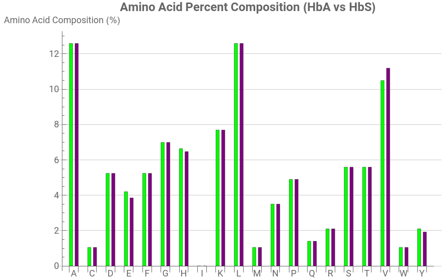


Looking at the broader picture across both proteins, the mutation does not significantly alter the overall amino acid composition of hemoglobin. Instead, the only noticeable difference is the substitution of glutamic acid (E) with valine (V). In normal hemoglobin (HbA), glutamic acid constitutes 4.20% of the amino acid composition, whereas in sickle-cell hemoglobin (HbS) it decreases to 3.85%. Conversely, valine increases from 10.49% in HbA to 11.19% in HbS. Every other amino acid remains unchanged, demonstrating that sickle-cell disease results from a single point mutation rather than widespread alterations to the protein sequence. This comparison illustrates how the replacement of just one amino acid can greatly impact the biological behavior of hemoglobin while leaving its overall amino acid composition largely unchanged. This can also be used to track amino acid abundance for various other diseases in order to decipher which specific change in amino acid abundance leads to a change in a proteins biological behavior giving rise to various threatening diseases.
This minor structural alteration observed between the two graphs also directly explains the painful physical symptoms of sickle cell anemia. Glutamic acid is highly polar and hydrophilic in nature which normally keeps the hemoglobin protein dissolved and stable in the blood plasma. When it is replaced by valine, a hydrophobic amino acid, a sticky patch is introduced on the protein and when oxygen levels drop these sticky patches lock into adjacent hemoglobin subunits to shield themselves from water, ultimately initiating a polymerization chain. The rigid protein rods then stretch across the red blood cells, wrapping the flexible biconcave disc into a fragile sickle shaped cell that blocks blood flow in microscopic capillaries (Kimball, 2016).
Analyzing Amino Acid Percent Composition by Secondary Structure
Analyzing Amino Acid Percent Composition by Secondary Structure
Extracting the Three Bio-Sequences (Helices, Sheets, and Loops)
Extracting the Three Bio-Sequences (Helices, Sheets, and Loops)
While analyzing the overall amino acid composition provides a broad overview of a protein’s sequence, it does not reveal how individual amino acids are distributed throughout the protein’s three-dimensional structure, since proteins are not uniform molecules. They are composed of distinct secondary structural elements that include the α-helices, β-sheets, and loop regions, each of which contribute differently to proteins structure. Since certain amino acids exhibit preferences for specific structural environments, examining the overall sequence may obscure some of the important compositional differences.
To automate this process, we developed a custom Wolfram function titled runExtractor to extract the amino acid sequences corresponding to each secondary structure element directly from a folded protein. Given a protein structure as an input, the function identifies all α-helices, β-sheets, and loop regions, and then returns three separate amino acid sequences: the helix string, containing the residues that form the alpha helix; the sheet string, containing residues that form the β-sheets; and the loop string, containing residues that do not belong to either of the structural regions.
By partitioning the complete protein sequence into its individual secondary structure components, each region can then be analyzed independently using the amino acid abundance functions developed previously. This also serves as the basis for comparing the compositional characteristics of various structural elements and enables the subsequent visualization through ternary plots.
findRanges extracts the list of integer coordinate pairs:
In[]:=
ClearAll[findRanges,findLoops];findRanges[data_,chain_]:=Cases[If[Head[data]===Association,Lookup[data,chain,{}],If[ListQ[data]&&Length[data]>=chain,data[[chain]],{}]],{_Integer,_Integer},All];
findLoops calculates the gap between the loop regions; Split groups the consecutive numbers in the loop together forming one single chain:
In[]:=
findLoops[totalLength_,helixPairs_,sheetPairs_]:=Select[Split[Complement[Range[totalLength],Flatten[Range@@@Join[helixPairs,sheetPairs]]],#2-#1==1&],Length[#]>0&];
fixSequence formats any variant of imported sequence data (list, or just string) and structures it into a chain-to-sequence map:
processChain cuts a single chain’s sequence into distinct secondary structure text strings using the calculated coordinate sets:
ExtractSequences downloads the raw PDB dataset, runs the function across each chain, and merges the aggregated results:
Final function (runExtractor) that executes the entire workflow on the specific target PDB IDs:
Extracting the raw data from the function to analyze the frequency of specific amino acids in the 3 bio-sequences respectively for both the mutated and normal variant of hemoglobin.
Mutated Helix:
Mutated Helix:
Mutated Sheet:
Mutated Loops:
Normal Helix:
Normal Sheet:
Normal Loops:
It is important to note here that in both cases (mutated and the normal protein) there is an empty data set for Sheets. This occurs because hemoglobin belongs to a specific structural class of proteins called as all-alpha proteins. Each of its four constituent subunits is formed exclusively by an arrangement of eight tightly bundled α-helices stabilized by intervening, non-repetitive loop segments. Because the classic β-pleated sheet is entirely absent from the topological design of hemoglobin the algorithm flags zero-sheet associated residues with it.
Graphing the Data using a Bar Graph
Graphing the Data using a Bar Graph
Defining the variables:
Initializing aminoAcids that contain the 20 standard amino acids in the protein, and setting this up as a reference list:
Creating two distinct variables to set up the dataset:
Lookup checks the target association data for each structure and returns an empty list if cannot be found; runs for helix, string, and loops in both mutated and normal variants:
LetterCounts runs through the entire combined sequence strings analyzing each character and returns the frequency of each individual residue:
Comparing our letter counts against aminoAcids and replacing missing entries with 0; map ensures any 0 values are substituted with 1
GraphicsRow takes both the charts and puts them side by side; the standard bar chart function is used to build the bar plots from the given coordinates and all characteristics have been defined:
Analysis of the Double Bar Graph
Analysis of the Double Bar Graph
Looking at both charts, the most striking feature is that neither graph shows any blue (β-sheet) segments at all as every bar is composed entirely of purple (helix) and green (loop) regions. This is fully consistent with the known biology of hemoglobin because it is a classic “all-α” globin fold, meaning essentially none of its 141 (α-chain) or 146 (β-chain) residues adopt β-sheet conformations, regardless of whether the protein is in its normal (HbA) or mutated (HbS) form.
When comparing helix/loop ratios residue-by-residue, most amino acids show only modest shifts between HbA and HbS . For example, alanine (A) is ~98% helical in HbA versus ~92% in HbS, and valine (V) is nearly identical in both forms at ~85% helix. This makes sense biologically, since a single amino acid substitution out of roughly 146 residues in the β-chain would not be expected to restructure the protein’s overall secondary structure composition since hemoglobin’s fold is highly conserved regardless of the mutation. However, a few residues do show more pronounced differences. Glutamic acid (E) drops from about 88% helix in HbA to roughly 73% helix in HbS, while phenylalanine (F) and histidine (H) show smaller comparable dips as well. This is particularly important given that the sickle cell mutation is itself a substitution of glutamic acid for valine at position 6 of the β-globin chain (E6V) but the graphs suggest that glutamic acid residues elsewhere in the mutated protein are also slightly less helix-favoring on average, which may reflect subtle downstream conformational effects of the mutation propagating beyond the single substituted site, even though the overall α-helical character of the protein is preserved. Tyrosine (Y) is the most loop-enriched residue in both variants (~33-50% loop), suggesting it consistently occupies flexible, non-helical turn regions in both HbA and HbS, regardless of the mutation.
Overall, the comparison supports the idea that HbS retains hemoglobin’s fundamentally α-helical secondary structure and supports the fact that the E6V mutation is a surface substitution that primarily disrupts intermolecular electrostatic interactions and promotes polymerization under deoxygenated conditions, rather than an internal change that would break down the protein’s core helical fold. The data here reinforces that sickle cell disease arises not from a wholesale change in hemoglobin’s secondary structure, but from a localized, chemically specific substitution whose effects become prominent at the molecular level rather than fundamental secondary-structure composition.
Creating the Ternary List Plot
Creating the Ternary List Plot
Comparing the Abundance of Amino Acids in the Three Sequences using a Ternary List Plot
Comparing the Abundance of Amino Acids in the Three Sequences using a Ternary List Plot
While standard bar charts provide a clear view of the absolute amino acid percent composition they fail to calculate the proportional behavioral shifts across multiple structural domains simultaneously. To evaluate how the sickle cell mutation destabilizes or preserves specific structural environments a ternary list plot can be implemented. The ternary plot maps three variables onto an equilateral triangle which comprise of coordinates such that their sum always adds up to 1.0 (or 100%). By calculating the absolute difference in amino acid distribution between normal hemoglobin and mutated sickle hemoglobin this visualization maps the exact structural locus of mutational impact on the protein. It allows for the instant determination of whether a given residue’s chemical environment was altered primarily within the rigid alpha-helix core, the flexible loop regions, or if it forced new beta sheets with amino acids to form (“How Do I Use Ternary Diagrams?”).
Defining all the variables and the sequence of 20 amino acid characters for reference:
normalData and mutatedData looks up the string key; StringJoin takes the broken text pieces and joins them as one string; LetterCounts counts the abundance of each character; and map is used to apply it to all 3 bio-sequences:
Normalize scales the math values so total = 1.0; Absolute value drops any negative signs; subtracts normal counts from mutated counts; double square brackets ensures only to take the helix and loop data:
Select filters out the data points and only retains the ones that are true:
Ordering checks for the largest value in the dataset; then checks if the dominant coordinate matches the index i; runs it thrice; Length measures the amount of elements to check inside if they are populated:
Using the Ternary List Plot to generate the graph; defining all the characteristics of the graph:
Analysis of the Ternary List Plot
Analysis of the Ternary List Plot
Most of the amino acid dots are purple and cluster heavily toward the right side of the baseline (Change in Helix > 0.5). This means that when comparing the normal and mutant PDB structural models, the overall absolute shifting that occurs takes place mostly inside the internal segments (which are within the rigid alpha helices). This goes in accordance with previous findings because helices make up the vast majority of hemoglobin’s mass. There are a few green dots that are further towards the left (Change in Loop > 0.5) and these represent specific amino acids whose behavior was disproportionately concentrated in the unstructured loop regions.
The distribution pattern of the amino acids observed in the ternary plot allows for the explanation of the physical mechanisms of sickle cell anemia. Sickle cell anemia is caused by a single point mutation as explored previously, and this occurs on the exterior surface of the protein which the code maps as the loop/surface data. Because the internal helices (the purple dots) remain largely unchanged in their structural positions the individual mutant hemoglobin unit (the monomer tetramer) keeps its shape. However the new hydrophobic valine out on the surface loop sticks and these sticky patches on different hemoglobin units latch onto one another. They eventually link up into forming a massive, rigid polymer chain fiber. This fiber is what physically stretches and distorts the red blood cells into the sickle shape which clogs capillaries and causes oxygen deprivation.
Conclusion
Conclusion
This study highlights the value of analyzing proteins at the secondary structural level rather than relying solely on complete amino acid sequence comparisons. By separating hemoglobin into α-helices, β-sheets, and loop regions, the computational workflow revealed how sequence variations are distributed within different structural environments. The analysis of healthy and sickle-cell hemoglobin showed that the mutation-associated changes were primarily localized within α-helical regions, while β-sheet regions remained highly conserved and loop regions showed limited variation. This pattern further reflects the structural stability of hemoglobin despite the presence of a disease-associated mutation and demonstrates how computational methods can decipher visual relationships between sequence changes and structural consequences. The developed Wolfram Language framework can be further applied to other proteins to investigate how molecular-level variations contribute to biological function and disease mechanisms.
Future Directions
Future Directions
The computational workflow we developed in this project provides a strong foundation for future studies of protein structure and function. Future work could extend these methods to larger and more diverse protein datasets, enabling comparisons across different biological pathways and disease states. The framework could also be enhanced by incorporating statistical analyses, such as principal component analysis (PCA) and clustering techniques, together with additional structural properties including solvent accessibility, residue conservation, hydrophobicity, and residue flexibility to provide deeper insight into protein molecules. Furthermore, machine learning algorithms such as Random Forests, Support Vector Machines, and Neural Networks could be integrated to classify proteins or predict the effects of disease-causing mutations. Ultimately, this computational model could be applied to a wider range of disease-associated proteins, including those implicated in Alzheimer’s disease, Parkinson’s disease, cystic fibrosis, and cancer, providing a versatile platform for investigating the relationship between protein sequence, structure, and function.
References
References
◼
Berman, H. M. (2000). The Protein Data Bank. Nucleic Acids Research, 28(1), 235–242. https://doi.org/10.1093/nar/28.1.235
◼
Clinic, C. (2025, June 24). What Are Proteins? Definition, Types & Examples. Cleveland Clinic. https://my.clevelandclinic.org/health/body/proteins
◼
How Do I Use Ternary Diagrams? (2023, August 11). Math You Need. https://serc.carleton.edu/mathyouneed/geomajors/ternary/index.html
◼
Kimball, J. (2016, July 13). 15.3I: Sickle-Cell Disease [Review of 15.3I: Sickle-Cell Disease]. Biology LibreTexts. https://bio.libretexts.org/Bookshelves/Introductory_and_General_Biology/Biology_(Kimball)/15%3A_The_Anatomy_and_Physiology_of_Animals/15.03%3A_Circulatory_Systems/15.3I%3A_Sickle-Cell_Disease
◼
Mandal, A. K., Mitra, A., & Das, R. (2020). Sickle Cell Hemoglobin. Subcellular Biochemistry, 94(94), 297–322. https://doi.org/10.1007/978-3-030-41769-7_12
◼
Modeling, N. R. C. U. C. C.-A. (1987). Secondary Structure of Proteins and Nucleic Acids. In Www.ncbi.nlm.nih.gov. National Academies Press (US). https://www.ncbi.nlm.nih.gov/books/NBK218568/
◼
Smith, Y. (2017, May 23). Amino Acids and Protein Sequences. News-Medical.Net. https://www.news-medical.net/life-sciences/Amino-Acids-and-Protein-Sequences.aspx
◼
Google. (2025). Gemini [Large language model]. https://gemini.google.com
Acknowledgments
Acknowledgments
I would like to express my sincere gratitude to Stephen Wolfram for providing the opportunity to explore this research topic and for his continued encouragement and guidance throughout the project. I am especially grateful for his insights that shaped the direction of this work and inspired the computational approach used in this study. I would also like to thank my mentor, Renata Toro, for her guidance and support throughout this project, Dr. Jason Sonnenberg for his assistance in mapping out the project and developing the computational methods, William Choi-Kim for his guidance during the initial planning stages, and the teaching assistants Max Wang, Averyl Xu,, Daniel Chengmin Xu, and Aanya Gupta for their valuable support in structuring and reviewing the computational essay.
Additional thanks to Stephen Wolfram for suggesting this project.
CITE THIS NOTEBOOK
CITE THIS NOTEBOOK
Analyzing secondary structural propensities in Hemoglobin through ternary graphing
by Misshka Sidhwani
Wolfram Community, STAFF PICKS, July 9, 2026
https://community.wolfram.com/groups/-/m/t/3751417
by Misshka Sidhwani
Wolfram Community, STAFF PICKS, July 9, 2026
https://community.wolfram.com/groups/-/m/t/3751417