ORIGINAL ARTICLE: Binous, H., Al-Mutairi, E. and Faqir, N. (2014), Study of the separation of simple binary and ternary mixtures of aromatic compounds. Comput. Appl. Eng. Educ., 22: 87-98. DOI: https://doi.org/10.1002/cae.20533
We consider an ideal equimolar binary mixture of benzene and toluene at . This mixture, with a thermal quality equal to 0.5, is fed to a 10-stage column with a total condenser and partial reboiler. The feed stage is stage 7. The feed flow rate is taken equal to . We set the values of the reflux ratio and reboil ratio equal to 3 and 2.5, respectively.
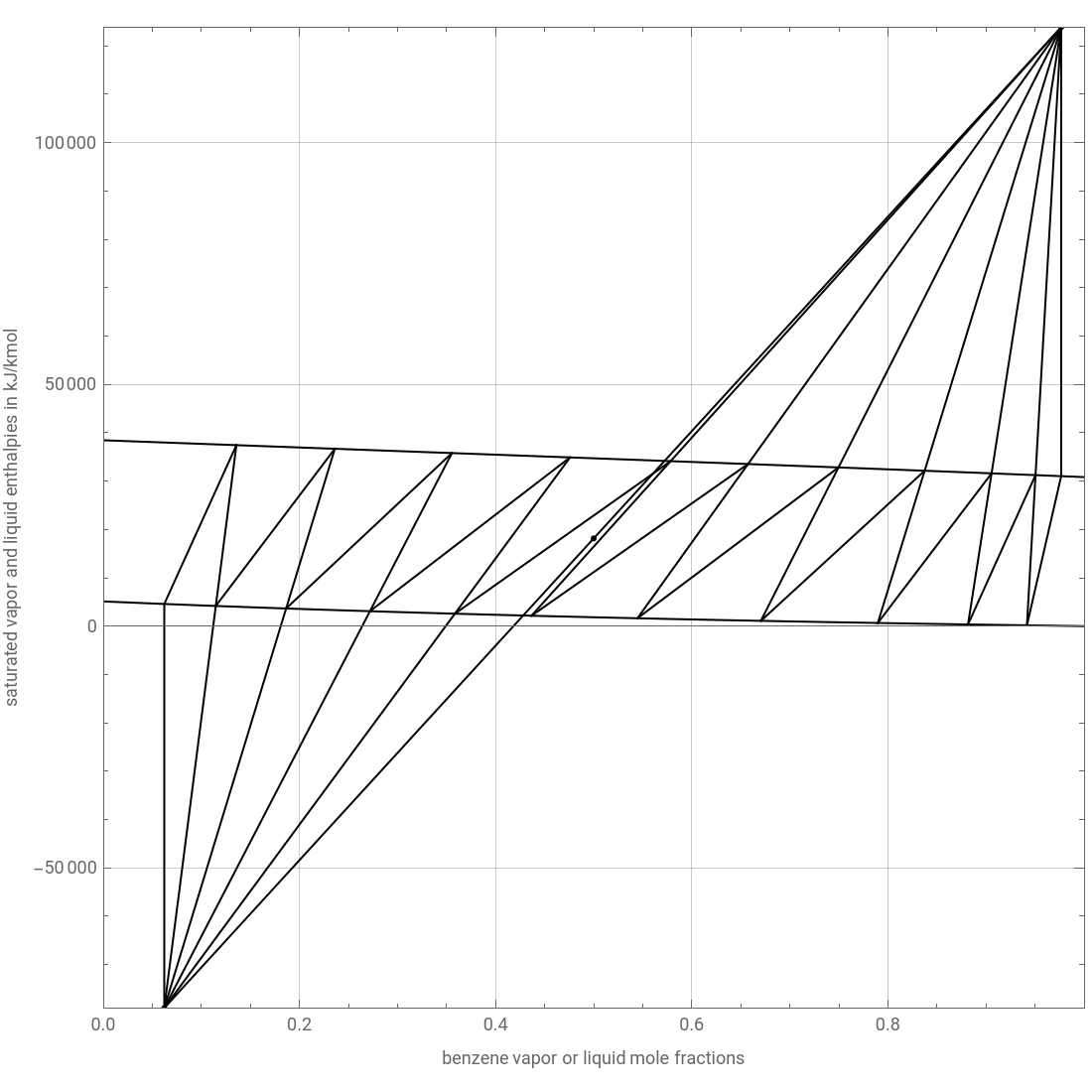
We computes the temperature and composition profiles using a rigorous approach, which includes both energy and mass balances. It is clear that the numerical simulation gives data similar to the graphical method developed by Ponchon–Savarit. The molar flow rate profiles for both the liquid and vapor phases are also displayed.
Our calculation showed that, for and , stage 7 is the optimal feed location. Indeed, if one changes the feed location while keeping the same values for and , the cooling and heating duties will be higher. The simulation finds cooling and heating duties equal to and , respectively, for and .
All results presented here show perfect agreement with those given by HYSYS (http://www.aspentech.com/hysys/).
760mmHg
10kmol/hr
R
s
We computes the temperature and composition profiles using a rigorous approach, which includes both energy and mass balances. It is clear that the numerical simulation gives data similar to the graphical method developed by Ponchon–Savarit. The molar flow rate profiles for both the liquid and vapor phases are also displayed.
Our calculation showed that, for
R=3
s=2.5
R
s
Qc=-592708kJ/hr
Qr=435526kJ/hr
R=3
s=2.5
All results presented here show perfect agreement with those given by HYSYS (http://www.aspentech.com/hysys/).
Total Pressure expressed in mmHg
In[]:=
P=760;
Antoine constants and equation
In[]:=
Aa1=6.90565;Ba1=1211.033;Ca1=220.79;Aa2=6.95464;Ba2=1344.8;Ca2=219.482;Psat1=10^(Aa1-Ba1/(T+Ca1));Psat2=10^(Aa2-Ba2/(T+Ca2));
Equilibrium constants. We consider that the mixture obeys Raoult’s law since benzene and toluene are both aromatic compounds.
K1=Psat1/P;K2=Psat2/P;
Feed composition
Benzene = component 1
Toulene = component 2
Benzene = component 1
Toulene = component 2
In[]:=
z1=0.5;z2=0.5;
Feed thermal quality -
In[]:=
phi=0.5;
Feed temperature, TF and composition
In[]:=
sol=FindRoot[(K1-1)z1/(1+(K1-1)phi)+(K2-1)z2/(1+(K2-1)phi)0,{T,100}];y1z=(K1)z1/(1+(K1-1)phi)/.sol;x1z=z1/(1+(K1-1)phi)/.sol;y2z=(K2)z2/(1+(K2-1)phi)/.sol;x2z=z2/(1+(K2-1)phi)/.sol;TF=T/.sol;
Feed enthalpy
hF=1/2(x1z(138.2(TF-80.1))+(1-x1z)(167.5(TF-80.1))+y1z(+96.3(TF-80.1))+(1-y1z)(+138.2(TF-80.1)));
λ
A1
λ
B1
VLE data for the binary mixture at 760 mmHg
In[]:=
i=0;While[i≤101,{xa=(i-1)0.01,sol=FindRoot[Psat1xa+Psat2(1-xa)P,{T,10,200}];xe[i]=xa,ye[i]=Psat1xa/P/.sol,Te[i]=T/.sol,i++}];Tbl1=Table[{xe[i],Te[i]},{i,1,101}];Tbl2=Table[{ye[i],Te[i]},{i,1,101}];Tbl3=Table[{xe[i],ye[i]},{i,1,101}];Tx=Interpolation[Tbl1,InterpolationOrder1];(*bubbletemperaturein°C*)Ty=Interpolation[Tbl2,InterpolationOrder1];(*dewtemperaturein°C*)xy=Interpolation[Tbl3,InterpolationOrder1];(*VLEdata*)
Latent heats of vaporization for benzene and toluene
In[]:=
λ
A1
λ
B1
Liquid and vapor phase enthalpy
In[]:=
He[y_]:=y(+96.3(Ty[y]-80.1))+(1-y)(+138.2(Ty[y]-80.1));he[x_]:=x(138.2(Tx[x]-80.1))+(1-x)(167.5(Tx[x]-80.1));
λ
A1
λ
B1
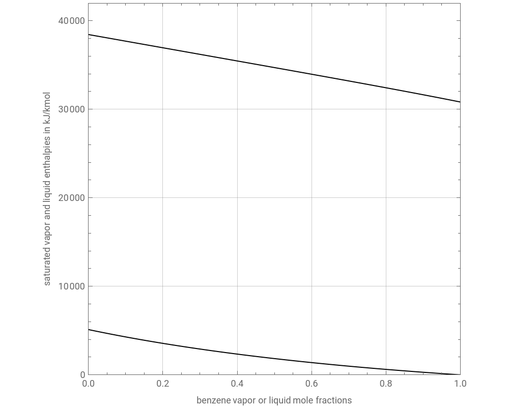
Ponchon-Savarit diagram or Enthalpy-Composition diagram
In[]:=
plt=Quiet[Plot[{he[x],He[x]},{x,0,1},FrameTrue,GridLinesAutomatic,ImageSize{500,400},PlotRange{{0,1},{0,42000}},PlotStyleThick,FrameLabel{"benzene vapor or liquid mole fractions","saturated vapor and liquid enthalpies in kJ/kmol"},AspectRatio1]]
Out[]=
Feed composition
In[]:=
zF=0.5;
Liquid and vapor enthalpies at stage i
In[]:=
H[i_]:=y[i](+96.3(T[i]-80.1))+(1-y[i])(+138.2(T[i]-80.1));h[i_]:=x[i](138.2(T[i]-80.1))+(1-x[i])(167.5(T[i]-80.1));
λ
A1
λ
B1
Vapor pressures at stage i
PSat1[i_]:=10^(Aa1-Ba1/(T[i]+Ca1));PSat2[i_]:=10^(Aa2-Ba2/(T[i]+Ca2));
MESH equations (mass and enthalpy equations)
In[]:=
Without loss of generality, we set R=3 and s=2.5. You can try out other values of R and s
In[]:=
R=3;s=2.5;
We call FindRoot in order to solve the MESH equations (a total of 60 nonlinear algebraic equations must be solved)
In[]:=
sysofEquations={eq3,eq4,eq5,eq6,eq7,eq8,eq9,eq10,eq11,eq12,eq13,eq14,eq15,eq16,eq17,eq18,eq19,eq20,eq21,eq22,eq23,eq24,eq25,eq26,eq27,eq28,eq29,eq30,eq31,eq32,eq33,eq34,eq35,eq36,eq37,eq38,eq39,eq40,eq41,eq42,eq43,eq44,eq45,eq46,eq47,eq48,eq49,eq50,eq51,eq52,eq53,eq54,eq55,eq56,eq57,eq58,eq59,eq60,eq61,eq62};
In[]:=
Length[sysofEquations]
Out[]=
60
In[]:=
sol1=Quiet@FindRoot[{eq3,eq4,eq5,eq6,eq7,eq8,eq9,eq10,eq11,eq12,eq13,eq14,eq15,eq16,eq17,eq18,eq19,eq20,eq21,eq22,eq23,eq24,eq25,eq26,eq27,eq28,eq29,eq30,eq31,eq32,eq33,eq34,eq35,eq36,eq37,eq38,eq39,eq40,eq41,eq42,eq43,eq44,eq45,eq46,eq47,eq48,eq49,eq50,eq51,eq52,eq53,eq54,eq55,eq56,eq57,eq58,eq59,eq60,eq61,eq62},{x[1],0.99},{x[2],0.93},{x[3],0.87},{x[4],0.76},{x[5],0.63},{x[6],0.50},{x[7],0.45},{x[8],0.37},{x[9],0.28},{x[10],0.12},{x[11],0.06},{y[1],0.99},{y[2],0.97},{y[3],0.94},{y[4],0.89},{y[5],0.82},{y[6],0.72},{y[7],0.67},{y[8],0.5},{y[9],0.37},{y[10],0.24},{y[11],0.13},{L0,173},{L1,162},{L2,160},{L3,138},{L4,135},{L5,184},{L6,183},{L7,182},{L8,190},{L9,182},{L10,182},{V1,191},{V2,190},{V3,188},{V4,186},{V5,183},{V6,132},{V7,133},{V8,133},{V9,132},{V10,132},{V11,132},{Di,4.7},{B,5.3},{T[0],80},{T[1],82},{T[2],81},{T[3],83},{T[4],87},{T[5],91},{T[6],92},{T[7],95},{T[8],98},{T[9],102},{T[10],105},{T[11],117},{Qc,-5.310^6},{Qr,410^6},MaxIterations10000]
Out[]=
{x[1]0.941738,x[2]0.881682,x[3]0.789683,x[4]0.670483,x[5]0.544642,x[6]0.436576,x[7]0.358468,x[8]0.271877,x[9]0.186401,x[10]0.114693,x[11]0.0621672,y[1]0.976665,y[2]0.95051,y[3]0.90571,y[4]0.837462,y[5]0.749605,y[6]0.657376,y[7]0.578444,y[8]0.475907,y[9]0.355459,y[10]0.236068,y[11]0.135703,L014.3631,L114.2768,L214.1384,L313.9489,L413.7395,L513.5598,L613.439,L718.3631,L818.2902,L918.2501,L1018.2431,V119.1507,V219.0644,V318.9261,V418.7366,V518.5272,V618.3475,V718.2267,V813.1508,V913.0779,V1013.0378,V1113.0308,Di4.78768,B5.21232,T[0]80.5699,T[1]81.287,T[2]82.5604,T[3]84.6177,T[4]87.4975,T[5]90.8407,T[6]94.0026,T[7]96.4814,T[8]99.4462,T[9]102.627,T[10]105.516,T[11]107.777,Qc-592708.,Qr435526.}
In[]:=
x[0]=y[1]/.sol1;(*distillatecompoisionassumingtotalcondenser*)
Ponchon-Savarit diagram
In[]:=
Show[plt,Graphics[{Thick,RGBColor[0.48,0,0],Table[Line[{{x[i],h[i]}/.sol1,{y[i],H[i]}/.sol1}],{i,1,11}],Thick,RGBColor[0,0.48,0],Table[Line[{{x[i],h[i]}/.sol1,{y[i+1],H[i+1]}/.sol1}],{i,1,10}],Thick,Cyan,Table[Line[{{y[i],H[i]}/.sol1,{y[1],(H[4]V4-h[3]L3)/Di}/.sol1}],{i,1,7}],Thick,Cyan,Table[Line[{{x[i],h[i]}/.sol1,{x[11],(h[8]L8-H[9]V9)/B}/.sol1}],{i,7,11}],Thick,Black,Line[{{x[11],(h[8]L8-H[9]V9)/B},{y[1],(H[4]V4-h[3]L3)/Di}}/.sol1],Magenta,PointSize[0.025],Point[{y[1],(H[4]V4-h[3]L3)/Di}/.sol1],Point[{zF,hF}],Point[{x[11],(h[8]L8-H[9]V9)/B}/.sol1]}],PlotRangeAll,AspectRatio1,ImageSize{550,550}]
Out[]=
Composition profiles
Temperature profile
Liquid and vapor phase flow rates
Flow rate profiles
CITE THIS NOTEBOOK
CITE THIS NOTEBOOK
Study of the separation of simple binary and ternary mixtures of aromatic compounds
by Housam Binous and Ahmed Bellagi
Wolfram Community, STAFF PICKS, January 14, 2024
https://community.wolfram.com/groups/-/m/t/3103062
by Housam Binous and Ahmed Bellagi
Wolfram Community, STAFF PICKS, January 14, 2024
https://community.wolfram.com/groups/-/m/t/3103062